Rubis is a game-changing, data-centric, bottom-up, history-matching tool. The decision to build Rubis came from looking closely at the way today’s engineers were working. KAPPA has chosen to be diametrically opposed to the development of the next generation of simulators which can handle zillions of cells with massive parallel processing. The objective is to match production data, as often and quickly and simply as possible, using the pieces of the jigsaw puzzle from the different methodologies. Rubis sits somewhere between single cell material balance and massive simulation models. It replaces neither but does much of the work of both.

One can build simple 3-phase, 3D numerical models, intuitively with no special training. The focus is on interactively building the field as it looks or import the volumes and properties from geomodelers. The grid builds automatically. The engineer concentrates on the problem, keeps it updated and does not worry about how to construct the tool itself.

In v4.20 substantial improvements have been brought to address the very low permeability of shale gas and CBM problem, including the integration of stress dependence and the adaptation of the gridding to the local diffusivity. The import of reservoir geometries and properties from geomodelers (GRDECL, CMG) now includes the net-to-gross, and calculation of upscaled properties has been improved. The export of a Rubis sector to Saphir NL for pressure transient analysis now transfers the dynamic state of the simulation at the date of the extraction.

The main idea is that gridding is just a necessary nuisance. What we are interested in is the physical problem we want to simulate, and we want this physical problem to be complex enough to reproduce the main drives of the reservoir that will affect production but simple enough to be run with a very short time cycle; hours, days or weeks, not months or years.

The grid is built as a final step after the physical problem has been defined by the input of (1) the PVT, (2) the geometry, i.e. horizons and volumes, (3) the reservoir static properties, (4) the well geometries, (5) the well data and constraints. Then, and only then, (6) the grid is built and (7) the simulation is run.

1. Defining the PVT
Rubis’ numerical solver is compositional but the PVT used is black-oil or modified black-oil. The Rs and rs relations are turned into a composition ratio, providing the grounds for a compositional formulation. Internal correlations can be used and tuned to match measured values. Alternatively tables can be loaded.

2. Defining the reservoir geometry
The user defines the areal perimeter of the reservoir and the number of geological layers. Individual layer volumes are defined by drawing or importing horizons and thickness fields. Internal faults can be defined. Scarce information is compensated for by kriging interpolation. As soon as the volumes are defined vertical cross-sections can be created and viewed.

3. Defining the reservoir properties
A default set of properties is defined, including petrophysical, which may be constant or areal, relative permeability / capillary tables and fluid contacts. Other sets of properties may be redefined and assigned to different layers and reservoir areas. In addition to the usual static properties, nonDarcy flow, doubleporosity, vertical and horizontal anisotropy may be defined. Each segment of the reservoir boundary can be set individually to sealing, constant pressure, or connected to various types of aquifers.

2+3. Importing geometry and properties
The interactive build may be replaced by an import from a geomodeler or another simulator using GRDECL or CMG format. In v4.20 the mapping of the limits and properties has been improved and now includes the net-to-gross. It is also possible to drag-and-drop a case, or part of a case, from another Rubis document or from a Saphir NL or Topaze NL numerical model.

4. Defining the well geometry
A well in Rubis may be either vertical, vertical with a hydraulic fracture, horizontal in a given layer ie: following the horizon of that layer, or slanted. Any number of perforations can be created and their opening/closing time defined individually. Each perforation may have a discrete skin which may be constant, rate dependent or time dependent. Because a wellbore model can be coupled with options including classical empirical, mechanistic and drift flux models, the well definition is not limited to its actual path in the reservoir. It is therefore possible to define the complete well trajectory from surface.

5. Defining the well data and constraints
Real well pressure and rate data can be loaded and edited. PDG and production data may be used and dynamically updated from Diamant Master. The user can define individual well model or import it from Amethyste. Controls can be constant or time dependent. Abandonment rates may be specified.

6. Building the grid
The unstructured Voronoi numerical model is common to Saphir NL, Topaze NL and Rubis, only local grid refinement around the wells will be different. The grid forms automatically and with the minimum number of cells. However, if required, the user may take full control.

7. Running the simulation
The user can override the default time range, solver settings, list of output results and frequency of the simulation restarts. Relevant output plots are created, pressure and saturation fields are initialized, and the individual well indices are calibrated from a hidden PTA grid. The simulation is then started and may be paused at any time. Individual plots are updated while the simulation is running. Information on the simulation process are also displayed in the lower message window.

Individual well production and pressures, together with reservoir statistical information, are displayed on a dedicated vs. time plot and updated in real time during the simulation. In playback mode, a vertical line highlights the active replay time.

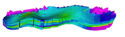
Static fields such as permeability or porosity and dynamic fields, such as pressures and saturations, can be displayed in 3D or 2D with vertical, horizontal or cross-section truncation.

A simulated production log, per well, showing the contribution by phase and zone is generated and time stepped in playback mode.

All data, input and stored, is organized in a hierarchical data browser. Any number of runs can be stored in a given session to enable what-ifs to be run.

The desorption models originally developed for Saphir NL and Topaze NL are available in Rubis, as well as the multi-fractured horizontal well and, in v4.20, stress dependency. Substantial improvements have been added in v4.20, including the adaptation of the individual well grid to the local value of the diffusivity and the expected simulation time steps.

When a shut-in has been identified in the pressure history, usually from a PDG measurement, the Rubis user may select a period of time and a section of the reservoir that will be transferred to Saphir NL. In v4.20 the state of the dynamic properties at the start of the extracted period is also sent to Saphir NL, hence the starting point is not the equilibrium but the ‘real’ state of the reservoir properties.

A complete Saphir NL document is initiated and the extracted build-up can be analyzed using the standard Saphir NL tools (specialized plots, analytical model or built-in numerical model) or driving the complex three-phase Rubis model, including gravity.

In Rubis v4.20 there is a temporary, experimental implementation of a full field thermal model developed in cooperation with TOTAL. Furthermore, a surface network module is included. These are for evaluation purposes only and can be activated for interested users by contacting KAPPA.