Basic HTML Version


OH – ET – VA - LL: Analysis of Dynamic Data in Shale Gas Reservoirs – Part 1 – Version 2 (December 2010)
p 12/24
The comparison remains more than acceptable when both well and fractures are gridded (i.e.,
when the 3D numerical model is built):
8 – Single fracture and no desorption
We continue with a single fracture case, in order to identify how nonlinearities affect the
quality of the different modelling and analysis techniques.
In order to hit two birds with one stone, we will not model one of the individual fractures of our
reference case, but a single equivalent infinite conductivity fracture with the total half length of
the fractured horizontal well, i.e. X
f
=10*200 ft = 2,000 ft. This is the solution currently
suggested in the industry to analyse horizontal wells with multiple fractures.
The other parameters and the production history follow the reference case description given in
§3. We consider the real gas diffusion and we no longer use pseudopressures.
We still ignore desorption for the time being.
We will now compare the “right” simulation with Topaze NL using our reference permeability of
1E-4 md, and we will compare it to the equivalent analytical model using pseudopressures
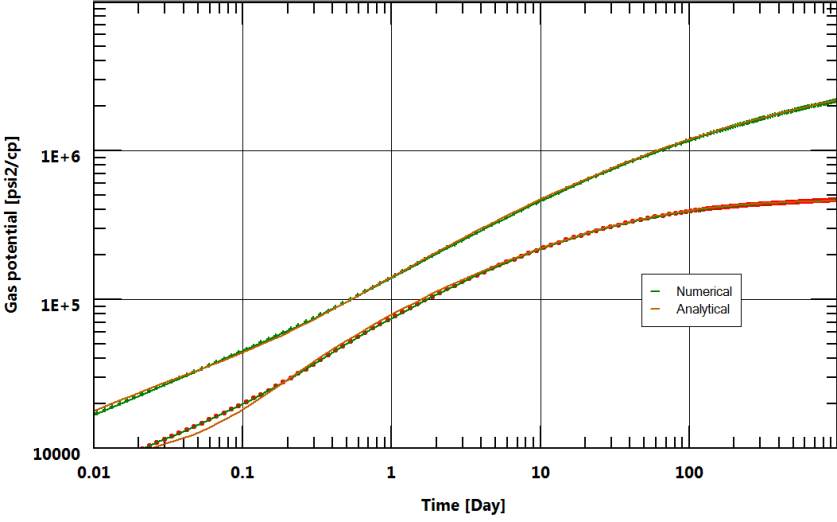
instead of the real gas diffusion. The result is seen in the loglog plot below.
The analytical model does not agree with the Topaze NL run anymore. Thanks to the high
pressure gradients and the corresponding changes in the gas compressibility, the numerical
model leads to estimates of final cumulative production that are approximately 15% higher
than for the analytical solution.
We then run a nonlinear regression on the analytical model to match the numerical case. After
regression the match is pretty good, but the estimate of k.X
f
2
after the match is 65% higher
than the original values.