Basic HTML Version


OH – ST - ET: Analysis of Dynamic Data in Shale Gas Reservoirs – Part 2
p 11/18
After refinement we get a shorter Xf around the lower end of the fracture half length
estimates, and a lower permeability: for a kh = 0.0072 md.ft, we have k = 7.2e-5 md. That is
reasonable as estimation, especially when significant uncertainties can lie within shale
permeability and fractures lengths. We also have little change in skin and an increase of
fracture number by one; this is within acceptable uncertainties range.
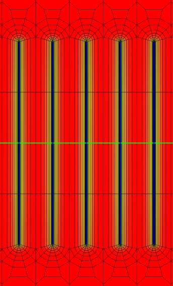
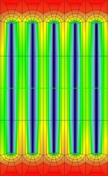
Since we are running a numerical simulation, we can observe the change of pressure over time
in the numerical grid. The pressure range varies from red (max) to blue (min) and we are
comparing an early time (after one month) production snapshot (left) with the final production
time one (right):
Pressure field after one month and 8 months
At early time, each fracture is producing as if independent, but after a few months of
production, we are transiting towards an interference regime where fractures are interacting
with each other. This verifies what we explained earlier in our analytical MFHW model.
Let us now make a 10-year forecast and compare it against the previous analytical models:
We see that the numerical one gives a better cumulative production compared to the analytical
MFHW one, but is still very much lower than the single fracture cumulative production forecast.
A note for the drainage area limitation: this shale gas play has such low mobility that in fact
most drainage is happening in the immediate vicinity of the well, thus it does not make a
difference whether to enclose the well within a bigger or smaller drainage area for forecasting,
since we do not impact the reservoir once further away from the fractures. More on this in a
later section of this paper.