Basic HTML Version


OH – ET – VA - LL: Analysis of Dynamic Data in Shale Gas Reservoirs – Part 1 – Version 2 (December 2010)
p 9/24
6.2 - The 3D model
If we do not want to ignore the direct flow between the formation and the horizontal well, we
have to go full 3D. In the 2D-Map, the user interface is the same. The dialog is also the same,
but the flow option is set to produce through the fractures and the horizontal drain. The
vertical anisotropy and the vertical position of the horizontal drain in the formation then
become relevant parameters. When this is done the calculation of the grid takes place. It is
substantially longer than the nearly instantaneous calculation of the 2D grids. The display of
the cells on the 2D-Map is actually a cross-section of the 3D grid at the vertical level of the
horizontal drain.
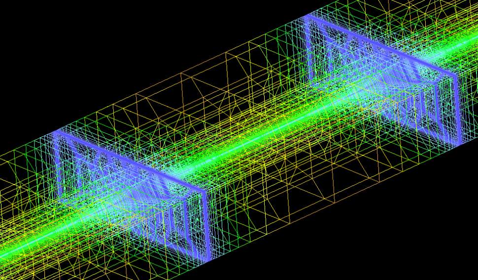
The figure below is the true 3D display of the gridding of our test case. For the sake of clarity
we have zoomed in on only a segment of the well in order to show two consecutive fractures.
The colour coding corresponds to the pressure gradient at the end of the four-year production.
Though it will be discussed later, the volume affected by the direct production to the horizontal
drain is relatively small.
It is relatively uncommon to encounter configurations where the well drain itself is perforated
in shale gas. For this reason we will not insist too much on this complex 3D grid geometry in
this document, but focus on the 2D geometry – where only the fractures are flowing.
Note that 3D gridding is also required when the fractures do not fully penetrate the formation,
although the gridding overhead in that case is less important than what is required in the full
well plus fractures gridding case.