Basic HTML Version


OH – ET – VA - LL: Analysis of Dynamic Data in Shale Gas Reservoirs – Part 1 – Version 2 (December 2010)
p 20/24
12 – Long time response and material balance plot
In all simulations we have assumed so far that the reservoir is infinite acting – boundaries
have been pushed far away in all numerical runs so that they could not interfere with the
pressure response.
Let us now consider a new case with desorption included and k=1E-4 md, with a highly
fractured horizontal well (100 fractures) sitting in the middle of a 5’000 square – the reason
why we need such a high number of fractures will become clear in a few lines:
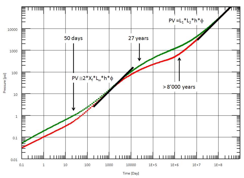
In the above, we let the simulation run until final pseudo-steady state flow could finally be
clearly visible, and it took a while: 100’000 years, with the final unit slope starting after 8’000
years. So forget about using the material balance plot to estimate actual shale gas reserves:
you will never see actual PSS in your lifetime (neither will your grand-grand-children). Note
that this result is not affected by the number of fractures, and that you still need plenty of
time (80 years to see PSS) if permeability is highered up to 0.01 md.
You will notice that data seem to bend towards pseudo-steady state flow much earlier in the
production history of this 100 fractures case: after about 50 days of production a “close to-”
unit slope is visible on the Topaze loglog plot, that remains for quite a long time (more than 20
years here). In fact if we inject these data in the material balance plot we recover a rough
estimate of the pore volume encapsulated by the fractures (or Stimulated Reservoir Volume,
SRV): 5191 Mscf, to be compared with 2.X
f
.h.L
w
.
4765 Mscf, where h is the reservoir
thickness and L
w
the well length.