Page 10 - Shale Gas Reservoirs Part 2

OH – ST - ET: Analysis of Dynamic Data in Shale Gas Reservoirs – Part 2

p 8/18

3.2 - Discussion

In the single fracture equivalent model, all fractures are represented by a single one.

Interaction between fractures is not taken into account.

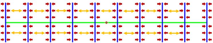
In the analytical model we take the real flow geometry into account. Interference happens

between nearby fractures, as all fractures start “competing”. Productivity decreases compared

to a system where fractures would be aligned side by side.

Schematic of interferences

During the first 8 months of production, the interference is negligible thanks to the very low

permeability of the system. Each fracture drains fluid separately from the other. This however

is not negligible anymore when planning a 10-year forecast, as we will move from an

independent linear flow for each fracture into a flow behavior where interferences are

dominating. Let us illustrate this in the log-log plot:

Comparison of the loglog response for both straight line and analytical models

The left hand side plot shows the single fracture equivalent model and the right hand side the

MFHW model. The log-log model is extended beyond data points as a 10-year forecast is made

in both cases.

We can see that although both models match reasonably well the data and look similar within

the data matching period, the flow behavior changes significantly later on: the single fracture

model continues its linear behavior, while the MFHW model shows that after 3000 hours the

slope increases due to interferences.

0.1

1

10

100

1000 10000

Time [hr]

10000

1E+5

1E+6

1E+7

Loglog plot: Int[(m(pi)-m(p))/q]/te and d[Int[(m(pi)-m(p))/q]/te]/dln(te) [psi2/cp] vs te [hr]

1

10

100