Basic HTML Version


OH – ST - ET: Analysis of Dynamic Data in Shale Gas Reservoirs – Part 2
p 7/18
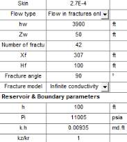
Loglog match and analytical model parameters after nonlinear regression
The parameters obtained from the match are within possible estimations of the well, we do
notice though that the fracture half-length falls into the high ends of the Xf estimates from our
preliminary estimations. We will get to an explanation later.
Both straight line and analytical model reasonably match the data. They differ completely
when we compare the 10-year forecast. The analytical model gives a significantly lower total
cumulative production and this could be critical for the economic value of the well.
Comparison of forecast for both straight line and analytical models
1
10
100
1000
Time [hr]
1E+5
1E+6
Integral of normalized pressure
Integral of normalized pressure Derivative
Loglog plot: Int[(m(pi)-m(p))/q]/te and d[Int[(m(pi)-m(p))/q]/te]/dln(te) [psi2/cp] vs te [hr]
0
2000
4000
6000
8000
10000
12000
14000
16000
Gas rate [Mscf/D]
0
1E+9
2E+9
3E+9
4E+9
5E+9
6E+9
7E+9
Gas volume [scf]
Equiv. Single fracture Xmf forecast
MFHW forecast
0
10000 20000 30000 40000 50000 60000 70000 80000 90000 1E+5
Time [hr]
2000
4000
6000
8000
10000
Pressure [psia]
Production history plot (Gas rate [Mscf/D], Pressure [psia] vs Time [hr])