Page 129 - Emeraude 2.60 Tutorial
Basic HTML Version

Emeraude v2.60 – Doc v2.60.01 - © KAPPA 1988-2010
Guided Interpretation #6
•
B06 - 9/13
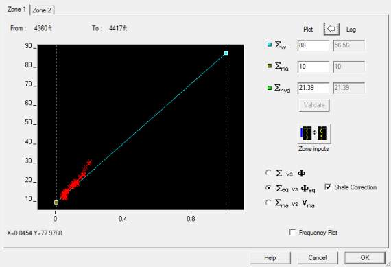
Fig. B06.15 • Cross-plots dialog
Note that you can also at this stage gauge the effect of the shale correction on this cross-plot
by toggling between the two options on the ‘Shale Correction’ checkbox.
Select the Cross-plot option:
ma
– V
ma
.
Select ‘Frequency plot’.
A grid is drawn on the plot, and a summation is made for each small square of the grid, giving
the total number of points inside the corresponding square on the plot.
On the
ma
– V
ma
cross-plot
ma is calculated by solving the
log equation in reverse,
assuming again that the saturations have not changed since initial times. The volume of
matrix, Vma, is Vma = 1 – Phie – Vsh. Hence on the plot the data points should funnel towards
the proper value of
ma for Vma = 1.
By moving the mouse cursor on the plot check that this is around a value of 11 c.u.
Modify the local value of
ma
and
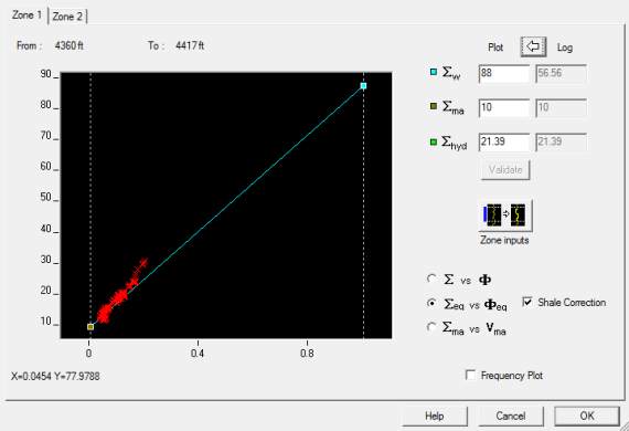
Fig. B06.16 • Cross-plots dialog
Make sure to use (and Validate) the following values:
w = 88 c.u.
ma = 11 c.u

