Page 149 - Emeraude 2.60 Tutorial
Basic HTML Version
Emeraude v2.60 – Doc v2.60.01 - © KAPPA 1988-2010
Guided Interpretation #8 • B08 - 5/25
Use the Show/Hide view dialog to set up the screen with VASPIFx views.
You can create a snapshot called ‘Vapps’ for this layout.
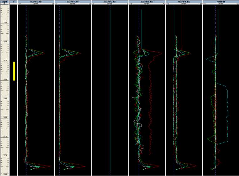
If the above steps were followed you should see that below 1455 m, and except for VASPIF3 in
pass D1 and up passes for VASPIF4, all FSI velocities are spot on (at 0).
Fig. B08.7 • Display of spinner apparent velocities
This is the spinner calibration that we will use to interpret the data in the flowing survey.
B08.2 • Flowing Survey: Handling Data
Create a new Survey called ‘Flowing’ with short name ‘Fl’. Enter the surface rates
[Qw=10m3/D, Qo=1600m3/D, Qg=465000 m3/D].
Load both Up files B08Up1.las and B08Up2.las (set the pass type to Up).
If needed, define the mnemonic ‘ACCE’ as ‘Always filtered’.
Import (some Gas holdup data are empty and therefore, not loaded).
Set the depth range to [3300m, 4000m]. You can set it as the default depth range.
Go to Survey-Tool info, and ensure that the blade diameter for SPIN is 0.064 m. Press OK.
In the flowing passes, some sensors were giving erratic measures: the corresponding data have
been removed from the LAS files to avoid tedious cleaning procedure for the user (note that the
‘Hide parts’ or ‘Delete parts’ options offer an easy way of doing it as shown next).
Again, in order to perform a quality control of the various tool readings, we will use the view
templates option.
In the Schlumberger templates, full layouts, call the following in turn (snapshots are created).

