Page 159 - Emeraude 2.60 Tutorial
Basic HTML Version


Emeraude v2.60 – Doc v2.60.01 - © KAPPA 1988-2010
Guided Interpretation #8 • B08 - 15/25
constraints. The 2D model parameters are evaluated by matching the reconstructed data on the
raw data, using a non linear regression.
Once obtained, the reconstructed values for the holdups and the velocities are combined to
calculate the local phase velocities. By integrating this information over the cross-section at every
depth, the average phase rates and holdups are produced, waving the need for slippage models.
These averages are then be used to feed a conventional PL interpretation.
Three 2D models are available for the FSI tool (linear, Mapflo and Prandtl) and as indicated
before, physical constraints can be added to the non linear regression: phase absence, vertical
segregation (e.g. water holdup decreasing from bottom to top), conventional tool measurements
(density, capacitance, spinner).
Click on ‘MPT processing’ (this interpretation option is enabled whenever MPT data have been
identified as such among the Survey log data).
Next to ‘Tool type’, click on the icon
to select the FSI measurements to be included in the
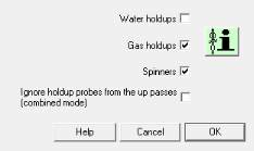
processing. Untick ‘Water holdups’ as it was decided to ignore the electrical probes.
Fig. B08.21 • Holdups selection
Select the 2DModel ‘Linear Velocity – MapFlo Holdups’. The
button on the same line allows
selecting the velocity extrapolation mode. Ensure that ‘0 at the pipe walls’ is selected, so the
fluid velocity profile will consider a null velocity at the pipe wall. The Mapflo 2D model forces
an areal average.
In Range, choose to process at ‘Interval’ with a value of 1m. This interval value also governs
the depth spacing for the averages.
In ‘Phase constraints’ impose the constraint ‘Yw =0’ as water production is negligible.
Choose to simulate VASPIN. A reconstructed VASPIN channel will be output to check for
consistency.
Select passes Up1 and Up2 in ‘Combined pass’ mode.
In combined mode, the readings of the selected passes are all matched simultaneously at each
depth, using the same 2D model: this mode behaves as if there was a FSI tool with twice the
number of probes. This can be of great interest when some probes failed in one pass but not in
another. Bear in mind that this mode is valid only if the flow conditions have not changed or are
very similar between the passes.

