Page 27 - Emeraude 2.60 Tutorial
Basic HTML Version
Emeraude v2.60 – Doc v2.60.01 - © KAPPA 1988-2010
Guided Interpretation #1
•
B01 - 25/38
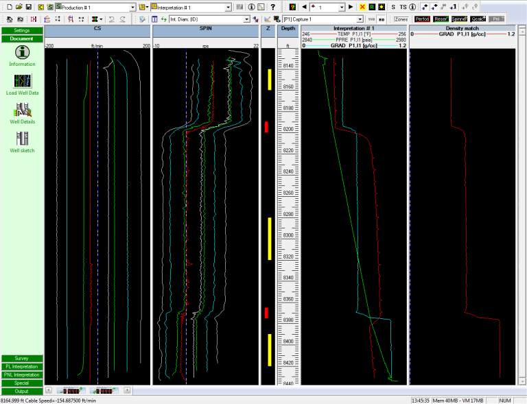
Fig. B01.30 • Calibration zones defined
Go to PL Interpretation tab and click on the ‘Calibrate’ icon.
The calibration plot is displayed (Fig. B01.31). Right click in the plot window and a zoom menu
is available. The active zone is highlighted in red. To activate a different zone, you may click
on the vertical schematic showing the 3 zones, or use the up / down arrows above. The slopes
and intercepts can be modified manually or copied from one zone to another. The two buttons
at the top labelled ‘Actions for all zones’ and ‘Actions for active zone’ give additional options.
In the
‘Actions for all zones’
button select: ‘Set all positive slopes to average’.
In the ‘Actions for all zones’ button select: ‘Set all negative slopes to average’.
Click on the ‘Thresh (+)’ button. A drop list to the right gives access to the possible no flow
zones. In this case there is only zone 3.
Select ‘Copy’ and the positive intercept value is copied as the tool threshold. Validate with OK.
Do the same for the negative threshold ‘Thresh (-)’.
For each line, an arrow pointing down shows the apparent velocity value for the positive line,
taking into account the positive threshold. Similarly, a line pointing up shows the value of
apparent velocity for the negative line. On zone 3, these two arrows coincide at 0 as we have
just defined the thresholds as the intercepts. This is not the case for zone 2. A difference in
those values could be due to a centralization problem and may well have to remain. If we
believe that the error is irrelevant we can unify all intercepts/slopes.
Make ‘zone 2’ active.
In ‘Actions for active zone’ select ‘Recompute zone with tool threshold’.

