Tutorial 3: Filtering data using external packages

The goal of this tutorial is to show the user a few additional aspects of the SDK that were introduced in the previous tutorials. One important aspect which was not covered was the use of external packages, such as SciPy . Additionally, we illustrate the use of the kappa_sdk.DataEnumerator class, which is useful when reading multiple data sources.

In this tutorial, we will filter and decimate noisy pressure and oil rate data. Before defining the input/output and script for our user task, we will first show the functions which will be employed.

The code for Tutorial 3 can be found in this zip file.

Starting point: tutorial_3_utility.py

Before writing the user task, we present a set of functions which we have available to perform the essential tasks that we desire. These functions are in tutorial_3_utility.py.

Click to view the contents of tutorial_3_utility.py

Listing 20 tutorial_3_utility.py - Filtering and decimation functions

import numpy as np
from scipy.ndimage import median_filter
from operator import itemgetter
from itertools import groupby
from typing import List


#  Filters pressures where rates are positive.
def filter_positive_values(rates: np.array, pressures: np.array, window_size: int) -> np.array:
    copy = np.copy(pressures)
    ranges = get_ranges_of_positive_values(rates)
    for r in ranges:
        if (r[1] + 1 - r[0]) < 4:
            continue
        #  Remove outlier peaks and valleys of 2 points or less
        pos_values = filter_peaks_and_valleys(pressures[r[0]:r[1] + 1], 2)
        size = min(window_size, (r[1] + 1 - r[0]) // 2 + 1)
        if size < 3:
            copy[r[0]:r[1] + 1] = pos_values
        else:
            copy[r[0]:r[1] + 1] = smooth(pos_values, size)
    return copy

#  Returns list of (start,end) indices for positive values of input vector
def get_ranges_of_positive_values(values: np.array) -> List[tuple]:
    ranges = list()
    for k, g in groupby(enumerate(values), lambda x: x[1] > 0):
        group = (map(itemgetter(0), g))
        group = list(map(int, group))
        if k:
            ranges.append((group[0], group[-1]))
    return ranges

#  Performs median filter of input data and replaces outliers using IQR criterion
def filter_peaks_and_valleys(data: np.array, size: int, iqr_mult: float = 1.5) -> np.array:
    window_size = 2 * size + 1
    if len(data) <= window_size:
        return data
    filtered = median_filter(data, window_size)
    diff_filter = data - filtered
    q1, q3 = np.quantile(diff_filter, [0.25, 0.75])
    iqr = q3 - q1
    diff_outlier_bools = np.logical_or(diff_filter > q3 + iqr_mult * iqr, diff_filter < q1 - iqr_mult * iqr)
    data_diff_filter = np.copy(data)
    data_diff_filter[diff_outlier_bools] = filtered[diff_outlier_bools]
    return data_diff_filter

#  Smooths input array x using numpy convolve (from Scipy Cookbook)
def smooth(x: np.array, window_len=11, window='hanning'):

    if x.ndim != 1:
        raise ValueError("smooth only accepts 1 dimension arrays.")

    if x.size < window_len:
        raise ValueError("Input vector needs to be bigger than window size.")

    if window_len < 3:
        return x

    if window not in ['flat', 'hanning', 'hamming', 'bartlett', 'blackman']:
        raise ValueError("Window is on of 'flat', 'hanning', 'hamming', 'bartlett', 'blackman'")

    s = np.r_[x[window_len - 1:0:-1], x, x[-2:-window_len - 1:-1]]
    # print(len(s))
    if window == 'flat':  # moving average
        w = np.ones(window_len, 'd')
    else:
        w = eval('np.' + window + '(window_len)')

    y = np.convolve(w / w.sum(), s, mode='valid')
    return y[(window_len // 2):-(window_len // 2)]


#  Calculates cumulative volumes assuming rates are in steps (at end)
def get_cum_volumes(time: np.array, rate: np.array):
    cum_volumes = np.zeros(len(time))
    for i in np.arange(1, len(time), dtype=int):
        delta_t = time[i] - time[i - 1]
        average_rate = rate[i]
        cum_volumes[i] = delta_t * average_rate + cum_volumes[i - 1]
    return cum_volumes


# Decimates the rates according to delta_t_max, respecting shut-in times and cumulative volumes
def get_decimated_times_rates(time, rate, delta_t_max):
    mid_point_times = list()
    mid_point_rates = list()

    cum_production = get_cum_volumes(time, rate)

    running_delta_t = 0
    running_delta_Q = 0
    for i in np.arange(len(rate) - 1, 0, step=-1, dtype=int):
        delta_t = time[i] - time[i - 1]
        running_delta_t += delta_t
        delta_cum = cum_production[i] - cum_production[i - 1]
        running_delta_Q += delta_cum

        record_rate = False
        # if-then conditions to record rate
        if i == 1:
            record_rate = True

        elif i > 0 and rate[i - 1] != 0 and rate[i] == 0:
            # First shut-in time
            record_rate = True

        elif i < len(rate) - 1 and rate[i + 1] == 0 and rate[i] != 0:
            # last rate before shut-in
            record_rate = True

        elif i > 0 and rate[i - 1] == 0 and rate[i] != 0:
            # first flowing time after shut-in
            record_rate = True

        elif i < len(rate) - 1 and rate[i + 1] != 0 and rate[i] == 0:
            # last shut-in time
            record_rate = True

        elif running_delta_t >= delta_t_max:
            # time difference is greater than maximum tolerance
            record_rate = True

        if (record_rate):
            mid_point_times.append(time[i - 1] + running_delta_t / 2)
            mid_point_rates.append(running_delta_Q / running_delta_t)
            running_delta_t = 0
            running_delta_Q = 0

    # end_point_times = end_point_times[::-1]
    mid_point_times = mid_point_times[::-1]
    mid_point_rates = mid_point_rates[::-1]

    slope = (mid_point_rates[1] - mid_point_rates[0]) / (mid_point_times[1] - mid_point_times[0])
    diff_t = mid_point_times[0] - time[0]
    rate_at_0 = mid_point_rates[0] - slope * diff_t
    mid_point_times.insert(0, time[0])
    mid_point_rates.insert(0, rate_at_0)  # mid_point_rates[0]) #

    slope = (mid_point_rates[-1] - mid_point_rates[-2]) / (mid_point_times[-1] - mid_point_times[-2])
    diff_t = time[-1] - mid_point_times[-1]
    rate_at_end = mid_point_rates[-1] + slope * diff_t
    mid_point_times.append(time[-1])
    mid_point_rates.append(rate_at_end)  # mid_point_rates[-1]) #

    return mid_point_times, mid_point_rates

Given these functions, we are ready to create our user task.

Defining the input

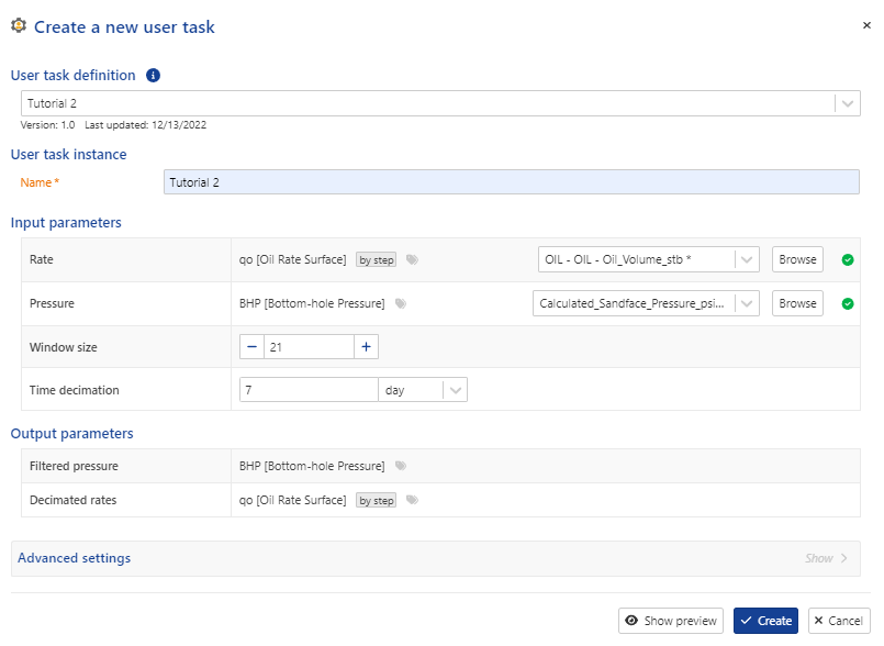
The input for this user task is shown below

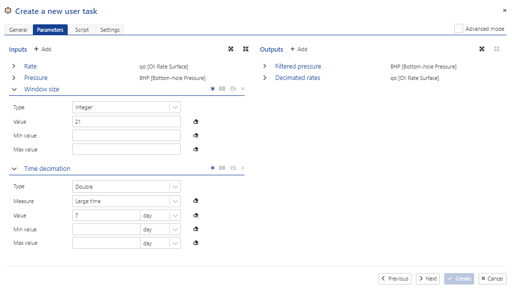
Fig. 19 The input for user task of Tutorial 3. This task requires pressures, oil rates, a window size (# of points)and the maximum times for decimation of the rate and pressure data.

The “Rate” and “Pressure” input parameters are self-explanatory. The “Window size” parameter is the number of points in the smoothing window. The “Time decimation” input is the maximum number of days to aggregate in the rate decimation. The equivalent .yaml description (see in the “Advanced mode” of Fig. 19).

Listing 21 The .yaml equivalent of the UI shown in Fig. 19

inputs:

    Rate:
      type: dataset
      mandatory: true
      dataType: qo
      isByStep: true

    Pressure:
      type: dataset
      mandatory: true
      dataType: BHP
      isByStep: false

    Window size:
      type:  int
      currentValue: 21
      mandatory: true

    Time decimation:
      type: double
      dimension: LargeTime
      currentValue: 168

outputs:


    Filtered pressure:
      type: dataset
      dataType: BHP
      isByStep: false

    Decimated rates:
      type: dataset
      dataType: qo
      isByStep: true

Writing the Python script

Reading in pressures and rates using the data_enumerator

As always, our Python script starts with some import statements, followed in this case by reading the data with a kappa_sdk.DataEnumerator instance.

Important

The kappa_sdk.DataEnumerator class is useful when reading multiple datasets.

from kappa_sdk.user_tasks.user_task_environment import services
import utility
import datetime
from scipy.interpolate import interp1d

services.log.info('Start of tutorial 3 user task')

data = services.data_enumerator.to_enumerable(
    [services.parameters.input['Rate'], services.parameters.input['Pressure']]) #  <==

The kappa_sdk.DataEnumerator.to_enumerable() method will accomplish many useful tasks. Most important is its treatment of the datasets when the dates are not identical, which is usually the case. The return object of kappa_sdk.DataEnumerator.to_enumerable() is a list of kappa_sdk.DataEnumeratorPoint instances. When the dates are different between datasets, kappa_sdk.DataEnumerator.to_enumerable() can return the union of all dates in the datasets, or just the dates associated with a reference dataset. It can also interpolate between data points, output all the points (including extrapolation of data), or just the points between common time ranges, etc. These options are all configurable using the kappa_sdk.DataEnumeratorSettings class in Python.

Settings for data_enumerator

In Tutorial 2, we did not describe the final tab of the user task creation UI. The “Settings” tab defines the default settings which will be passed to the user task script.

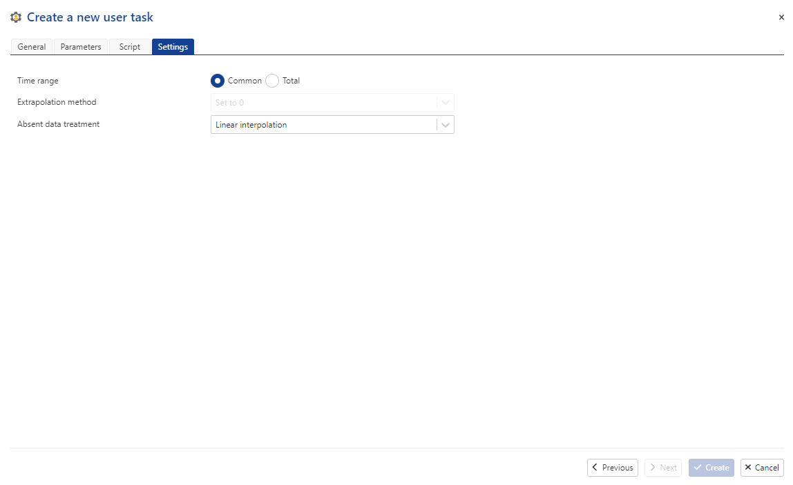
Fig. 20 The final tabbed pane of the user task definition UI specifies the default settings for the user tasks’s kappa_sdk.DataEnumerator instance.

The settings passed to the kappa_sdk.DataEnumerator instance are set when creating the user task.

In the script, the user can modify the default settings using kappa_sdk.DataEnumerator.get_default_settings(). This method will return a kappa_sdk.DataEnumeratorSettings instance which you can use to configure the kappa_sdk.DataEnumerator instance in the script (Listing 22).

Listing 22 Use of get_default_settings() to obtain an instance of the DataEnumeratorSettings

data_enumerator_settings = services.data_enumerator.get_default_settings()
#  Modify data_enumerator_settings below
  ...
  ...
data, _, _ = services.data_enumerator.to_enumerable(
    [services.parameters.input['Rate'], services.parameters.input['Pressure']], data_enumerator_settings)

The kappa_sdk.DataEnumeratorSettings class also allows you to define the start and end dates that kappa_sdk.DataEnumerator.to_enumerable() will return, as well as the amount of data which will be read in one call.

Warning

The return object of kappa_sdk.DataEnumerator.to_enumerable() depends on whether the data_enumerator_settings is passed. This may change in the future.

Processing the data

Since the pressure is point data and the rate is step data, it is important to understand what is returned by kappa_sdk.DataEnumerator.to_enumerable(). Below (Listing 23), the elements of the list data are read in a for-loopand the dates, rates, pressuresand elapsed times are stored in list objects.

Listing 23 Storing the data and calculating the elapsed times.

dates = list()
rates = list()
pressures = list()
times = list()
first_date = data[0].date
for point in data:
    dates.append(point.date)
    elapsed = (point.date - first_date).total_seconds() / 60.0 / 60.0
    times.append(elapsed)
    rates.append(point.values[0])
    pressures.append(point.values[1])

Point data like pressures have a data point at the start of the dataset. However, step data are often stored with the times (and corresponding rate values) recorded at the end of the step. What kappa_sdk.DataEnumerator.to_enumerable() does in this case is add the first point for the rates, with a rate value of 0. So in the example here, the first element of the “times” and “rates” lists will be 0.

Smoothing the pressure and rate data

The first goal of the user task is to smooth daily pressure data, but only when the well is producing. After smoothing, the user task will then decimate the pressure and rate data (while preserving the cumulative production). Using the code in “tutorial_2_utility.py”, we can do this in just a few additional lines of code (Listing 24).

Listing 24 Smoothing the pressures where rates are positive, then decimating the rates and pressures

#  Size of window for smoothing
window_size = services.parameters.input['Window size']
services.log.info('Smoothing pressure signal for non-zero rate periods')
filtered_pressures = utility.filter_positive_values(rates, pressures, window_size)

#  Time period for rate decimation
delta_t_max = services.parameters.input['Time decimation']

# # Decimate the rate values by delta_t_max (preserving cumulative production)
decimated_times, decimated_rates = utility.get_decimated_times_rates(times, rates, delta_t_max)

decimated_dates = list()
for t in decimated_times:
    new_date = first_date + datetime.timedelta(hours=t)
    decimated_dates.append(new_date)

pressure_interpolator = interp1d(times, filtered_pressures)
filtered_pressures = pressure_interpolator(decimated_times)
services.data_command_service.replace_data(services.parameters.output['Filtered pressure'], decimated_dates, filtered_pressures.tolist())

#  Step data requres the set_first_x method
services.data_command_service.set_first_x(services.parameters.output['Decimated rates'], decimated_dates[0])
services.data_command_service.replace_data(services.parameters.output['Decimated rates'], decimated_dates[1:], decimated_rates[1:])

Plotting the results

We would like to create a plot which compares the original vs decimated pressures and rates. We’ll do this using the Plot API (kappa_sdk.Plot and kappa_sdk.PlotChannel), which was introduced in Tutorial 1. In this example, we create a plot with two panes, one for the pressure comparison, the other for the rate comparison. Note the differences in how the kappa_sdk.Data instances are retrieved - they are different depending on whether the data are an output from the user task, or if the data are from the well. Note also how the kappa_sdk.Plot.add_data() method is called to specify the different panes. Finally, remember what was shown in Tutorial 1 - when kappa_sdk.Data instances are passed to the kappa_sdk.Plot.add_data() method, the plot only needs to be created onceand the results will automatically be updated when new data arrive.

Listing 25 Plotting the comparison between the original vs decimated pressures and rates

if plot is None:
    # The plot has not yet been created
    pressure_pane_name = 'Pressures'
    #  Create the plot under the user task "Plots" sub-node
    new_plot = services.user_task.create_plot(plot_name, pressure_pane_name)
    # Add the pressure data to the plot
    pressure_data = next(x for x in services.well.data if x.vector_id == str(pressure_vector_id))
    series_name = 'Original pressure'
    press_series = new_plot.add_existing_data(pressure_data, series_name, pressure_pane_name, show_symbols=True, show_lines=False)
    #  Add the filtered pressure data to the plot
    filtered_pressure_data = next(x for x in services.user_task.outputs
                                  if x.vector_id == str(services.parameters.output['Filtered pressure']))
    series_name = 'Filtered Pressure'
    filtered_press_series = new_plot.add_existing_data(filtered_pressure_data, series_name, pressure_pane_name, show_symbols=False, show_lines=True)
    filtered_press_series.set_lines_aspect(style=LineAspectEnum.solid)

    # Create a new pane
    rates_pane_name = 'Rates'
    new_plot.add_sub_plot(rates_pane_name)
    #  Add the rate data to the new pane
    rate_data = next(x for x in services.well.data if x.vector_id == str(rate_vector_id))
    rate_name = 'Original rates'
    rate_series = new_plot.add_existing_data(rate_data, rate_name, rates_pane_name, show_symbols=False, show_lines=True)
    # Add the decimated rate data to the new pane
    decimated_rate_data = next(x for x in services.user_task.outputs
                               if x.vector_id == str(services.parameters.output['Decimated rates']))
    rate_name = 'Decimated rates'
    decimated_rate_series = new_plot.add_existing_data(decimated_rate_data, rate_name, rates_pane_name, show_symbols=False, show_lines=True)
    decimated_rate_series.set_lines_aspect(style=LineAspectEnum.dash)
    # Plot the two panes
    new_plot.update_plot()

Simulating the user task in the SDK

We will run this user task with the SDK before creating the task in KAPPA-Automate. As we saw in Tutorial 1, this is done by creating the main simulation file. If the user task script is titled “tutorial_3_usertask.py”, we create a file entitled “tutorial_3_usertask_simulation.py”. Listing 26 shows the contents of the simulation file.

Listing 26 The file “tutorial_3_usertask_simulation.py”

from kappa_sdk import Connection
from kappa_sdk.user_tasks import Context
from kappa_sdk.user_tasks.simulation import UserTaskInstance


ka_server_address = 'https://your-ka-instance'
print('Connecting to {}'.format(ka_server_address))
connection = Connection(ka_server_address, verify_ssl=False)

field_name = 'your field name'
print("Reading [{}] field data...".format(field_name))
field = next(x for x in connection.get_fields() if x.name == field_name)

well_name = 'your well name'
print("Reading [{}] well...".format(well_name))
well = next(x for x in field.wells if x.name == well_name)

context = Context()
context.field_id = field.id
context.well_id = well.id

task = UserTaskInstance(connection, context)
print("  [->] Well Name = {}".format(task.well.name))

print('[Tutorial 3] Binding parameters..')
rate_data_type = 'qo'
rate_name_prefix = 'OIL - '  # 'Oil rate'
rate_data = next(x for x in task.well.data if x.data_type == rate_data_type and x.name.startswith(rate_name_prefix))
print("  [->] Rate Name = {}".format(rate_data.name))
task.inputs['Rate'] = rate_data.vector_id

pressure_data_type = 'BHP'
pressure_name_prefix = 'Calculated'  # 'BHP'
pressure_data = next(x for x in task.well.data if x.data_type == pressure_data_type and x.name.startswith(pressure_name_prefix))
print("  [->] Pressure Name = {}".format(pressure_data.name))
task.inputs['Pressure'] = pressure_data.vector_id

task.inputs['Window size'] = 21

task.inputs['Time decimation'] = 168

task.run()

Listing 26 uses the pressure and rate datasets from the Kite well of the SPE RTA database, a public set of data set up by the SPE in a 2020 workshop.

When we run the script in Listing 26 with “tutorial_3_usertask.py”, “tutorial_3_usertask.yaml”and “tutorial_3_utility.py” in the same directory, the output can be viewed in KAPPA-Automate under the “Gauges” folder.

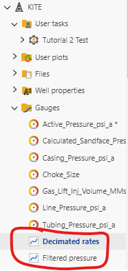
Fig. 21 The output of the user task can be viewed under the “Gauges” folder, circled in red.

Once the user task has been tested and validated using the SDK, we are ready to create the user task in KAPPA-Automate. To do this, a new package containing the file “tutorial_3_utility.py” must be created.

Creating a new package

In Tutorial 2, we learned how to create a user task from the “Automation” panels. One subject that was not covered was how to create a new package. In order to use the code in “tutorial_3_utility.py” in the user task in KAPPA-Automate, we need to zip the file and create a package in the KAPPA-Automate UI. Select the “Automation” icon just as one would to create a new user task, then click on “User tasks” in the left toolbar. Select the “Packages” tabbed pane as shown in Fig. 22.

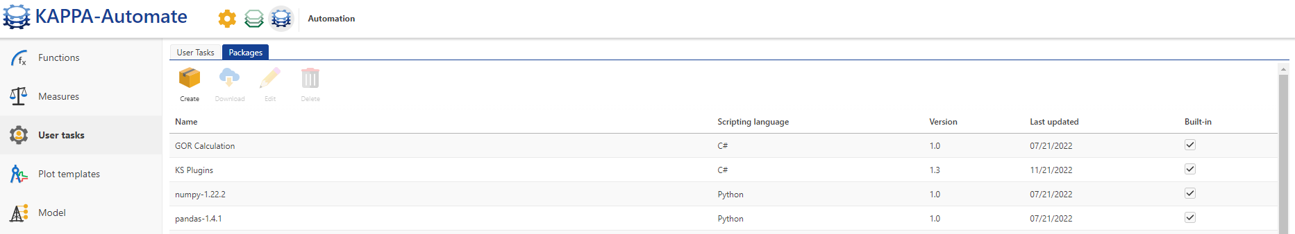
Fig. 22 The “Packages” tab is available after selecting the blue “Automation” icon. This tabbed pane allows the user to create, edit, delete or download packages.

Click on the “Create” button. This will bring up a UI dialog (Fig. 23). Here you can specify the name of the package (no restrictions on the name), the scripting language (Python), give the description of the packageand most importantly, upload the zip file containing the Python code.

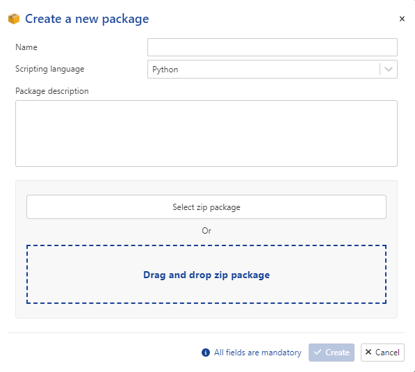
Fig. 23 Selecting the “Create” button displays the above UI. Zip files containing Python code are uploaded by dragging the file to the window, or by selecting the “Select zip package” button.

After uploading, the UI will resemble Fig. 24 below.

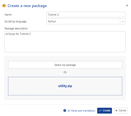
Fig. 24 After uploading the zip file, the UI will display the zip file name.

Select “Create” in Fig. 24 to create the new package. The package will appear in the list. Note that you are free to name the package whatever you wish - its name is only used for identifying the package in the input UI, shown below. In this tutorial, the zip file was created by right-clicking on the tutorial_3_utility.py file and zipping the file and naming it “utility.zip”.

The Python user task script

The contents of the script have been described above. The Python script created with the SDK has been copy/pasted in the “Script” window of the user script UI shown in Fig. 25 below. Note as well that the “Tutorial 3 Lib” package has been selected, containing the tutorial_3_utility.py code as shown in Listing 20. This package was added by selecting the “down-arrow” button next as indicated by the red arrow.

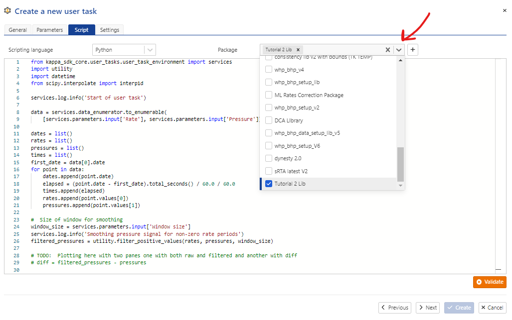
Fig. 25 The user task “Script” pane, showing the selection of the tutorial library package containing tutorial_3_utility.py (Listing 20). This package was added by selecting the “down-arrow” button next as indicated by the red arrow.

Before creating the user task, we also must add the Sci{y and NumPy packages. These packages are pre-installed in the embedded Python in KAPPA-Automate and should be found in the package list.

Below you can find the full user task code in one code block, for further understanding. Note on Line 2, the import of the tutorial_3_utility.py file.

Click to view the contents of tutorial_3_usertask.py

Listing 27 The full Python script for Tutorial 3

from uuid import UUID
from typing import List, cast
from kappa_sdk.user_tasks.user_task_environment import services
import tutorial_3_utility as utility
from datetime import datetime, timedelta
from scipy.interpolate import interp1d
from kappa_sdk import LineAspectEnum


services.log.info('[Tutorial 3] Start of user task')

rate_vector_id = cast(UUID, services.parameters.input['Rate'])
pressure_vector_id = cast(UUID, services.parameters.input['Pressure'])

data = services.data_enumerator.to_enumerable([rate_vector_id, pressure_vector_id])

dates: List[datetime] = list()
rates: List[float] = list()
pressures: List[float] = list()
times: List[float] = list()
first_date = data[0].date
for point in data:
    dates.append(point.date)
    elapsed = (point.date - first_date).total_seconds() / 60.0 / 60.0
    times.append(elapsed)
    rates.append(point.values[0])
    pressures.append(point.values[1])

#  Size of window for smoothing
window_size = cast(int, services.parameters.input['Window size'])
services.log.info('[Tutorial 3] Smoothing pressure signal for non-zero rate periods')
filtered_pressures_array = utility.filter_positive_values(rates, pressures, window_size)

#  Time period for rate decimation
delta_t_max = cast(float, services.parameters.input['Time decimation'])

# # Decimate the rate values by delta_t_max (preserving cumulative production)
services.log.info('[Tutorial 3] Decimate the rate values by {}'.format(delta_t_max))
decimated_times, decimated_rates = utility.get_decimated_times_rates(times, rates, delta_t_max)

decimated_dates = list()
for t in decimated_times:
    new_date = first_date + timedelta(hours=t)
    decimated_dates.append(new_date)

services.log.info('[Tutorial 3] Interpolate pressure')
pressure_interpolator = interp1d(times, filtered_pressures_array)
filtered_pressures: List[float] = pressure_interpolator(decimated_times).tolist()
services.data_command_service.replace_data(str(services.parameters.output['Filtered pressure']), decimated_dates, filtered_pressures)

#  Step data requires the set_first_x method
services.data_command_service.set_first_x(str(services.parameters.output['Decimated rates']), decimated_dates[0])
services.data_command_service.replace_data(str(services.parameters.output['Decimated rates']), decimated_dates[1:], decimated_rates[1:])

this_task = services.user_task
plot_name = 'Pressure/Rate Comparison'
plot = next((x for x in this_task.plots if x.name == plot_name), None)

if plot is None:
    # The plot has not yet been created
    pressure_pane_name = 'Pressures'
    #  Create the plot under the user task "Plots" sub-node
    new_plot = services.user_task.create_plot(plot_name, pressure_pane_name)
    # Add the pressure data to the plot
    pressure_data = next(x for x in services.well.data if x.vector_id == str(pressure_vector_id))
    series_name = 'Original pressure'
    press_series = new_plot.add_existing_data(pressure_data, series_name, pressure_pane_name, show_symbols=True, show_lines=False)
    #  Add the filtered pressure data to the plot
    filtered_pressure_data = next(x for x in services.user_task.outputs
                                  if x.vector_id == str(services.parameters.output['Filtered pressure']))
    series_name = 'Filtered Pressure'
    filtered_press_series = new_plot.add_existing_data(filtered_pressure_data, series_name, pressure_pane_name, show_symbols=False, show_lines=True)
    filtered_press_series.set_lines_aspect(style=LineAspectEnum.solid)

    # Create a new pane
    rates_pane_name = 'Rates'
    new_plot.add_sub_plot(rates_pane_name)
    #  Add the rate data to the new pane
    rate_data = next(x for x in services.well.data if x.vector_id == str(rate_vector_id))
    rate_name = 'Original rates'
    rate_series = new_plot.add_existing_data(rate_data, rate_name, rates_pane_name, show_symbols=False, show_lines=True)
    # Add the decimated rate data to the new pane
    decimated_rate_data = next(x for x in services.user_task.outputs
                               if x.vector_id == str(services.parameters.output['Decimated rates']))
    rate_name = 'Decimated rates'
    decimated_rate_series = new_plot.add_existing_data(decimated_rate_data, rate_name, rates_pane_name, show_symbols=False, show_lines=True)
    decimated_rate_series.set_lines_aspect(style=LineAspectEnum.dash)
    # Plot the two panes
    new_plot.update_plot()

services.log.info('[Tutorial 3] End of user task')

After selecting the necessary packages for the user task, click on the “Create” button to create the user task in KAPPA-Automate.

Creating the user task for a well

To create the user task for the well (Kite), we follow the same procedure as in Tutorial 2. Select the well node, then select the “User Task” icon in the toolbarand the user task UI will appear as shown below. Note that the mandatory dataset inputs have been already defined.

Clicking on the “Create” button will create the user task and queue the task for execution. When finished, the output in the “Plot” tabbed pane will resemble the figure below:

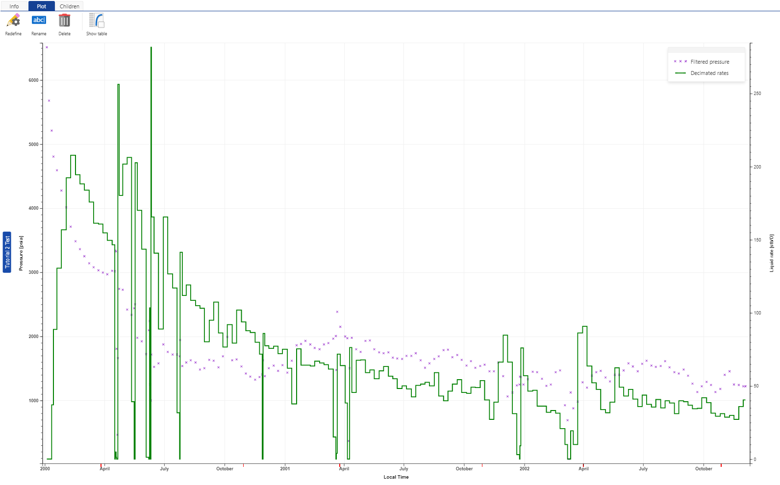
In the next tutorial, we will use these filtered and decimated rates and pressures as input to a Topaze file for well Kite.