Productivity Index Trend

Objectives

The objective of this workflow is to track the evolution of well Productivity Index (PI) with time and to break it into various terms, representative of the influence of PVT, completion, reservoir, etc. PI_model and its breakdown into multiple terms is a common output for both steady-state or PSS and transient models. In addition, raw PI is computed from a KA pressure gauge for transient models.

Theory

Steady state or PSS

For the steady state or pseudo steady state (PSS) models, PI_model can be expressed either as 𝑞/∆𝑃 or as a function of model parameters.

Equation 1.

PImodel=\frac{q}{\left(pbar-pwf\right)}=2\pi\frac{kh}{Bµf\left(s,..\right)}

Note

For gas cases, we replace pressure (p) with pseudo-pressure (m(p)). We then use gas formation volume factor (B), viscosity (µ), and total compressibility evaluated at p̄ if the user selects it as the input. Otherwise, we use pₑ for each shut-in.

As for total compressibility, it is recalculated from flash results using cr, sw, and cw, which are derived from well properties extracted from the Saphir file.

f(S,..) is a function of skin and drainage area geometry (size and shape / distances from well to boundaries). As f(S,..) could contain parameters whose values could not be estimated with sufficient confidence, PI_model for this case is calculated using the q/∆P equation.

The pbar in this equation comes from the Saphir file. Saphir computes Pbar for closed reservoirs using pore volume calculated from model boundary distances, cumulative production, and PVT parameters.

PI expression is a product of terms: PI=a.b.c and hence, log(NPI) takes the form log(a/a0) + log(b/b0) + log(c/c0). The log(NPI) for Steady state or PSS, normalized w.r.t values at time t0, can be expressed as below.

Equation 2.

\log\left(NPI\right)=\log\left(\frac{PImodel}{PImodel\left(to\right)}\right)=\log\left(\frac{k}{ko}\right)+\log\left(\frac{Boµo}{Bµ}\right)+\log\left(\frac{f\left(So,..\right)}{f\left(s,..\right)}\right)

The log normalized contributions of permeability and 𝐵𝜇 are computed using the corresponding properties whereas that of skin is computed using the equation below which contains PI_model computed using q/∆P.

Equation 3.

\log\left(\frac{f\left(So,..\right)}{f\left(S,..\right)}\right)=\log\left(\frac{PImodel}{PImodel\left(to\right)}\right)-\log\left(\frac{k}{ko}\right)-\log\left(\frac{Boµo}{Bµ}\right)

Transient radial

For the transient radial model, PI_model is expressed uniquely as a function of model parameters.

Equation 4.

PImodel=2\pi\frac{kh}{Bµ\left[\ln\left(re\left(\frac{∆t}{rw}\right)+S-\frac{1}{2}\right)\right]}

Note

For gas cases, we replace pressure (p) with pseudo-pressure (m(p)). We then use gas formation volume factor (B), viscosity (µ), and total compressibility evaluated at the reference pressure that users select (p_1hr or x hrs after shut-in).

As for total compressibility, it is recalculated from flash results using cr, sw, and cw, which are derived from well properties extracted from the Saphir file.

∆𝑡 is the elapsed time since the start of shut-in which is an input to the user task. The investigation radius at time ∆𝑡 is given by:

Equation 5.

re\left(∆t\right)=2\sqrt{\frac{k∆t}{µ\cdot phi\cdot ct}}

The components of log(NPI) for transient radial flow models are computed using the equation below.

Equation 6.

\log\left(NPI\right)=\log\left(\frac{k}{ko}\right)+\log\left(\frac{Boµo}{Bµ}\right)+\log\left(\frac{\ln\left(re\left(\frac{Δt}{rw}\right)+So-\frac{1}{2}\right)}{\ln\left(re\left(\frac{Δt}{rw}\right)+S-\frac{1}{2}\right)}\right)

For transient models, in addition to PI_model, a PI_rawTransient is computed using 𝑝𝑤𝑠(∆𝑡) from the pressure gauge under KA well.

Equation 7.

PIraw\left(t\right)=\frac{q\left(t\right)}{pws\left(Δt\right)-pwf\left(Δt\right)}

Transient linear and bilinear

Model
Transient Linear	Equation 8. $\frac{Bµ}{2\pikh}Sf+\frac{Bµ}{2\sqrt{\pi}xfkh}\left(\frac{k}{µ.phi.ct}\right)^{\frac{1}{2}}\left[tp^{\frac{1}{2}}+dt^{\frac{1}{2}}-\left(tp+dt\right)^{\frac{1}{2}}\right]$
Transient biinear	Equation 9. $\frac{Bµ}{2\pikh}Sf+\frac{\frac{2.451}{2\pi}Bµ}{\sqrt{Fck}kh}\left(\frac{k}{µ.phi.ct}\right)^{\frac{1}{4}}\left[tp^{\frac{1}{4}}+dt^{\frac{1}{4}}-\left(tp+dt\right)^{\frac{1}{4}}\right]$

Note

As for total compressibility, it is recalculated from flash results using cr, sw, and cw, which are derived from well properties extracted from the Saphir file.

𝑡𝑝 is the equivalent production time.

It is possible to normalize the individual terms in these equations w.r.t 1/PI (to):

Equation 10.

Normalizes\frac{1}{PI}=\frac{\frac{1}{PImodel}}{\frac{1}{PImodel\left(to\right)}}=\frac{1term}{\frac{1}{PImodel\left(to\right)}}+\frac{2term}{\frac{1}{PImodel\left(to\right)}}

For linear and bilinear models, 1/PI(t) is a sum of terms and hence, log(NPI) cannot be calculated for these models. However, it is possible to normalize the individual terms in these equations w.r.t 1/PI(t0). Here again, both PI_model and PI_rawTransient as computed as in the previous case.

Multiphase flow

If the analysis is multiphase (B𝜇)t and 𝜇t given by the Perrine equations below are used in place of B𝜇 and 𝜇 for all three cases.

Equation 11.

\left(Bµ\right)t=\frac{1}{\frac{kr0}{µ0B0}+\frac{kr}{µB}+\frac{krg}{µgBg}}

Equation 12.

µt=\frac{1}{\frac{kr0}{µ0}+\frac{kr}{µ}+\frac{krg}{µg}}

Input

Prerequisites

Before creating the user task, the engineer must ensure that a well property container with the following property values, depending on the model to be used, should exist:

Property	Steady state or PSS	Transient radial	Transient linear	Transient bilinear
Permeability, K	+	+	+	+
Reservoir thickness, h	+	+	+	+
Last flowing pressure, Pwf	+	+	+	+
Reference rate, q	+	+	+	+
Average pressure, Pbar	optional
Skin		optional	optional	optional
Well radius, rw		optional
Porosity, phi		optional	optional	optional
Total compressibility, ct		optional	optional	optional
Equivalent production time, tp			optional	optional
Fracture half length, xf			optional
Fracture conductivity, Fc				optional
Formation volume factor(s)	optional	+	+	+
Viscosity(ies)	optional	+	+	+

The easiest way to have the necessary property container filled with the properties values is to extract the properties from a Saphir document(s) to Master container.

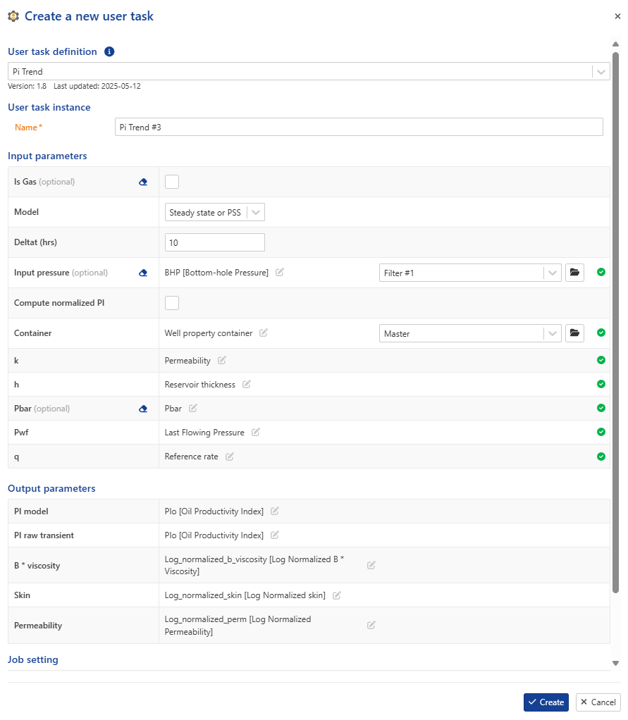
Model – The model used to derive the equation that computes the PI model. The current implementation can handle four different model types: Steady state or PSS, Transient radial, Transient linear and Transient bilinear.
Is Gas – Check this option to compute the PI trend for gas cases.
Gas PVT – This option appears only when Is Gas is selected, allowing the user to select the PVT object to be used in the user task.
Deltat (hrs) – Filtered pressure of data type “BHP”. This is an optional input for the transient models to calculate 𝑝𝑤𝑠(∆𝑡) that appears in the 𝑃𝐼𝑟𝑎𝑤(𝑡) equation. If this input is left empty PI raw transient will not be computed.
Input pressure (optional) – This is an optional input for the transient models used to calculate Pws (delta t) that appears in the PI raw (t) equation; if this input is left empty PI raw transient will not be computed and the corresponding output gauge will be empty. Last flowing pressure, Pwf(t), as well as average pressure, Pbar, for the delta P calculations are taken from the property container.
Report RealPI at 1 hour (optional) – Appears only if deltat equals to 1 hr.
If checked the user task reports the values of real Productivity index, P at 1 hour raw from the container otherwise values of at delta t =1 hr are calculated.
Container – The well property container from which well properties are read and computed PI results are written into.
Compute normalized PI – Specifies whether the log(NPI) terms or normalized 1/PI_model terms should be calculated and plotted. When checked, the user is obliged to provide a reference datetime for normalization.
Reference date – The well properties at this datetime will be used for normalization. If the specified datetime lies between two well properties, the values from the earlier well property will be used. If the specified date is before the first well property, the first well property in the time series will be used as reference.
Normalized PI will be calculated only for well properties after this reference date.
Note
In addition, there is a list of well properties that appear as inputs in the user task creation dialog. These input variables exist only to inform the user of the well properties used in the computation and their values are not accessed in the user task definition dialog. These properties are listed in prerequisites section above.

Output –

The user task outputs PI model (for all model types) and PI raw transient (computed only for transient models with valid input pressure) are added under the user task node.

In case if necessary input parameters for PI raw transient are absent the corresponding output gauge is empty. If “Real PI at 1Hour” is checked the values of the property container are reported as PI raw transient. Alternately, for transient models real PI could be computed for any delta t given valid input pressure gauge that lives in KA.

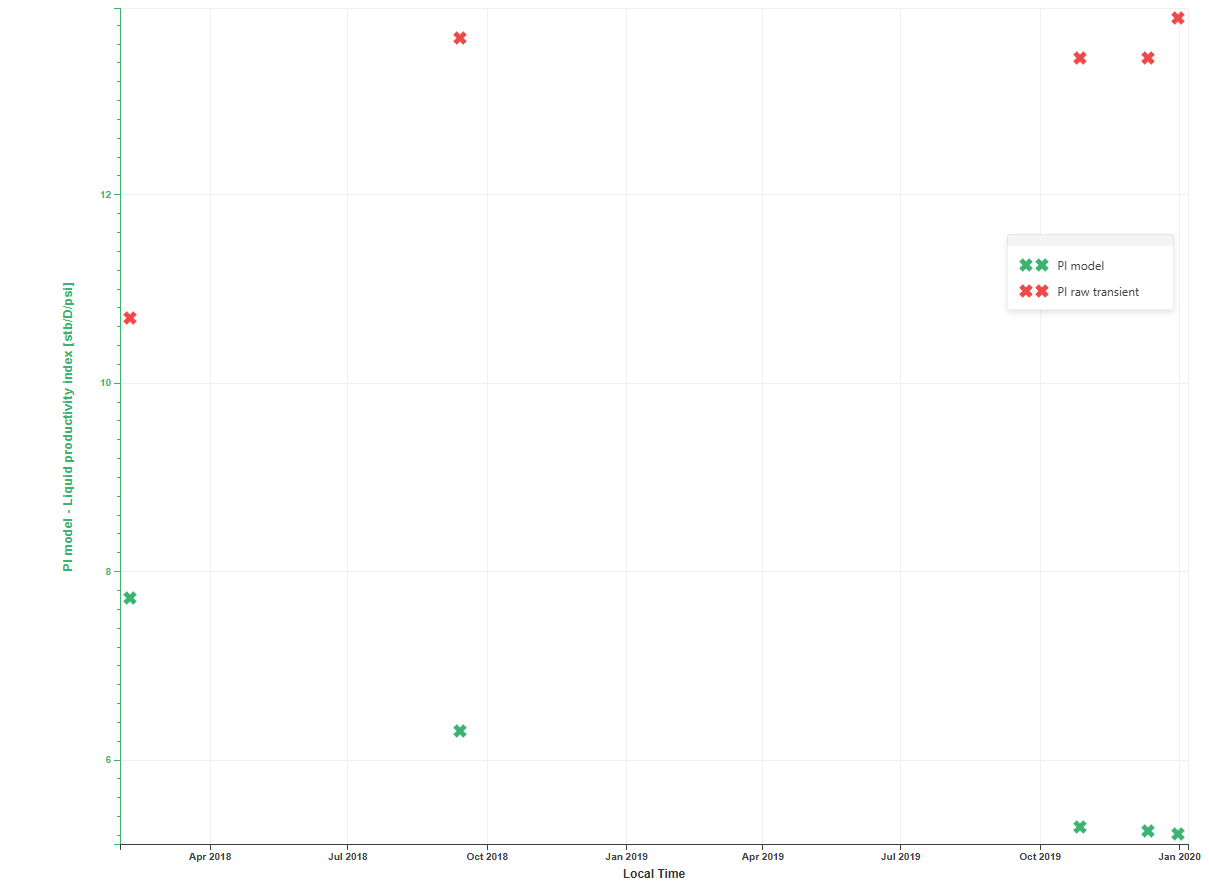
Output custom plot:

A custom histogram plot of PI_model (for steady state and PSS models) or PI_model and PI raw transient (for transient models) is created under the user task. If Compute Normalized PI is checked and a valid reference date is provided, a second pane with log(NPI) terms (for radial flow models) or normalized 1/PI terms (for linear flow models) is plotted as stacked bar charts and added to the custom plot.

User Task dialog

Output channels

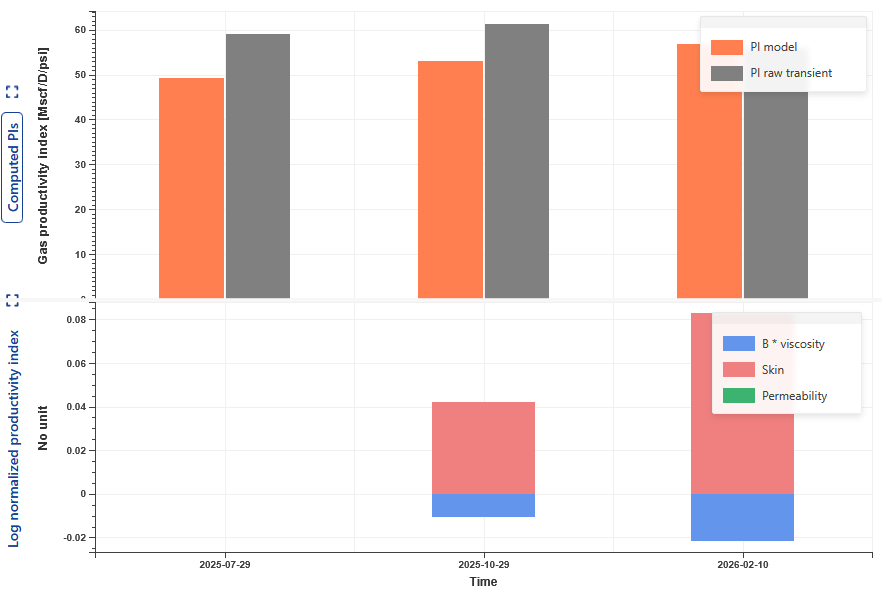
Chart bar plot

In this section:

K-A End User Help