Tutorial 1
This tutorial covers the entire PDG workflow, including both the basic and advanced sections, with a focus exclusively on the oil phase. You will learn how to create a PDG workflow from scratch; starting with creating a field and well, then loading and filtering the data, autmatically identifying shut-ins, generating iPTA workflow, and creating plot templates.
Creating a field
The highest-level object in the K-A hierarchy is a Field. A field can in turn contain wells, which can possibly be organized in well groups.
To create a field:
Connect to K-A from an internet browser using a web address provided by your IT support.
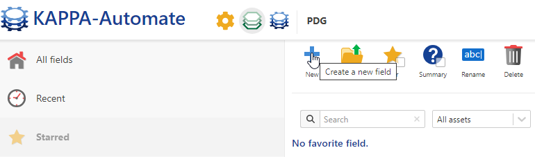
Click on New ,  .
.
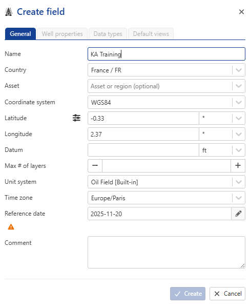
Change the Field Name to KA Training, keep all the other information as default.
Click on Create
 |
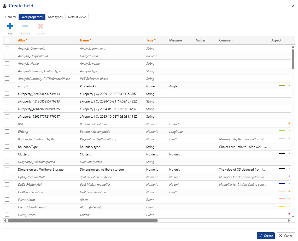
By switching to the second tab, you can view the complete catalog of Well Properties. If necessary, you can add a new Well property by clicking on . In this example, we will use the ones already available.
 |
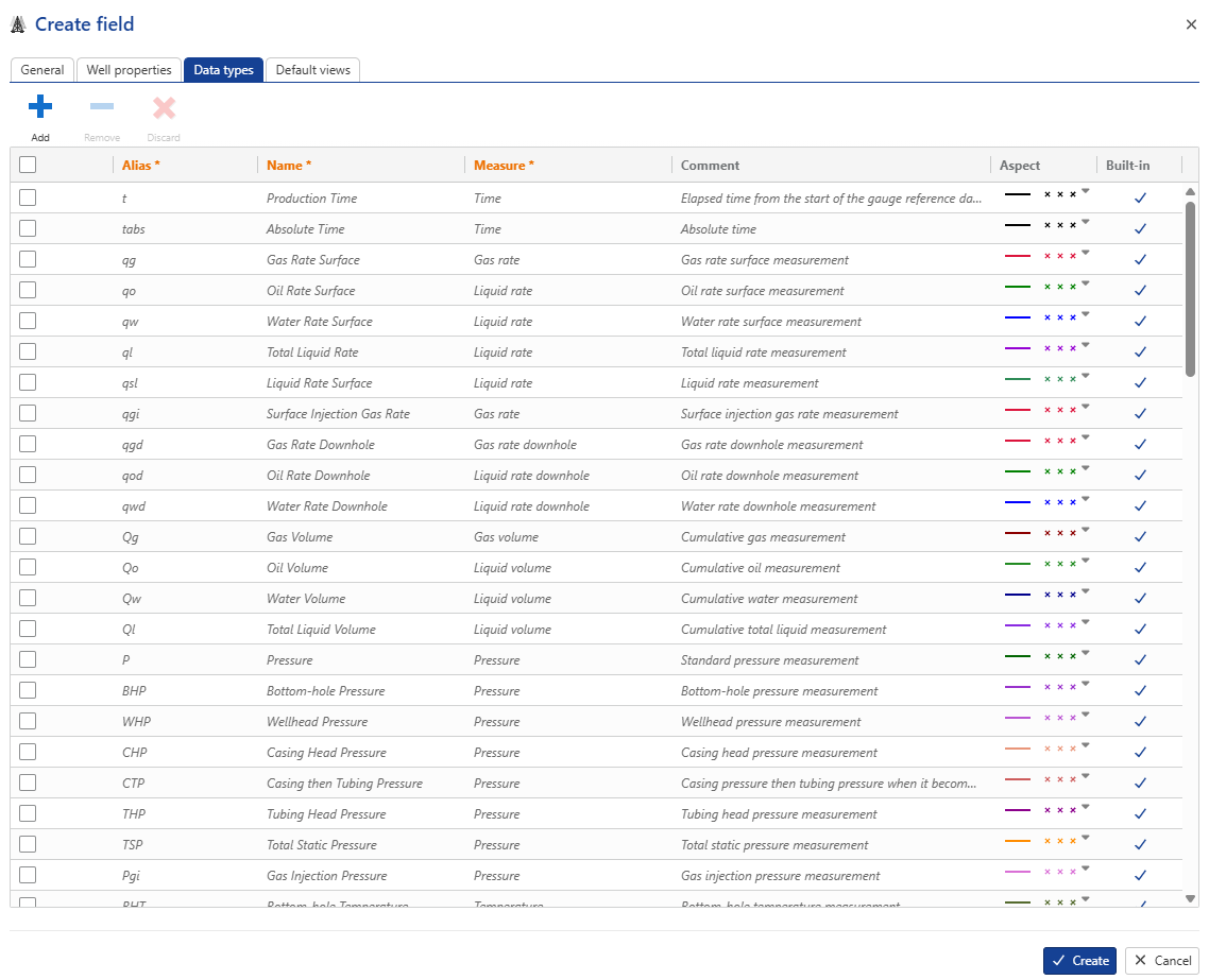
By switching to the third tab, you can also view the complete catalog of Data types. If necessary, you can add a new Data type by clicking on . In this example, we will use the ones already available.
 |
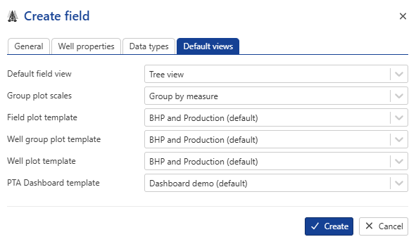
By switching to the last tab, you can define a default view, plot scales, and a template for this field on your local machine. Each time you open this field on the same machine, these settings will be retained.
 |
Creating a well
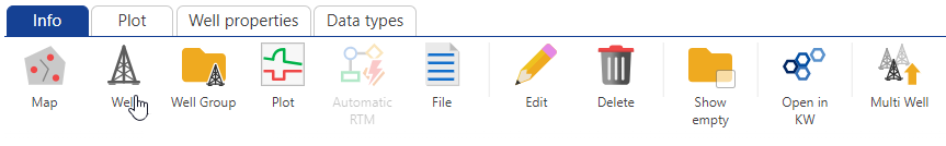
To add a well, select the field and under the Info tab, click on Well ,  , among the options listed at the top:
Change the well Name to KAEX01 , set Production type to Oil Producer, keep all the other information as default.
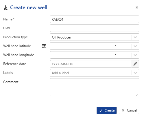 |
Press Create.
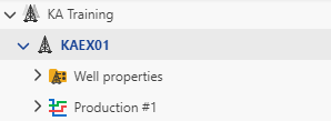
The well will be listed in the field hierarchy:
 |
Mirroring and Filtering Gauges
Gauges are used to store time lapse data. Once created, a Gauge automatically mirrors (copies) data from a tag located in a historian. Gauges can store data as points or steps.
Creating a Gauge
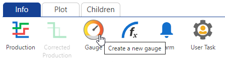
To create a gauge, select the well and under the Info tab, click on Gauge among the options listed at the top:
The Load window dialog prompts the user to select the data source. Select the BLI Gauges data source where the training datasets are located. Leaving the tag filters blank, click on  to display a list of all the gauges located in the data source:
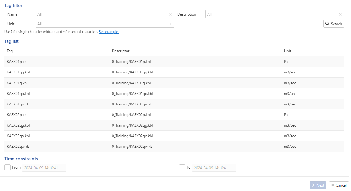 |
Data source connectors are predefined links to the company’s data Historian or KAPPA-Server installation and are set up by Administrators of the KAPPA Automate platform. For this exercise, we will be loading the following two gauges:
KAEX01p.kbl
KAEX01q.kbl
Loading Pressure data
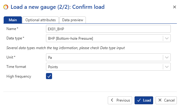
Select KAEX01p.kbl in the Tag list and click on Next. Change the gauge Name to EX01_BHP, Data type to BHP [Bottom-hole Pressure] :
 |
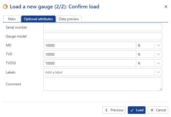
Switch to 'Secondary parametrs dialog and change and MD , TVD and TVDSS to 10000 ft:
 |
Click on Load.
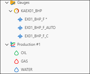
The gauge will be listed under a Gauges folder in the field hierarchy:
High and Low Frequency Gauges
At load time, KAPPA-Automate treats any source gauge (not being loaded under Production) as high frequency. This is denoted by the High frequency flag in Step 2 of the gauge loading process:
Any high-frequecy data also has an HF label on its icon in the field hierarchy. Users may manually uncheck this flag (usually not recommended) if they only wish to load part of the gauge with less than 100,000 points. However, as the gauge is updated with new data, as soon as the total number of points exceeds 100,000, KAPPA-Automate will automatically flag the gauge as High Frequency. This may have consequences on any workflows using this gauge.
When dealing with High Frequency Gauges, it is recommended not to use the raw gauges directly but filter them to the necessary level for a particular application. In fact, certain built-in workflows in KAPPA-Automate like Shut-In Identification, iPTA and iRTA etc., do no accept raw high frequency gauges as input. It is also not possible to transfer high frequency gauges to KAPPA-Workstation.
Gauge Preview
When loaded, the plot for a high frequency gauge does not show all gauge data. Like in K-S, only a representative preview of the full gauge is shown on the contextual plot. However, it is possible to show a slice (of 100,000 points) of the raw gauge data on the plot.
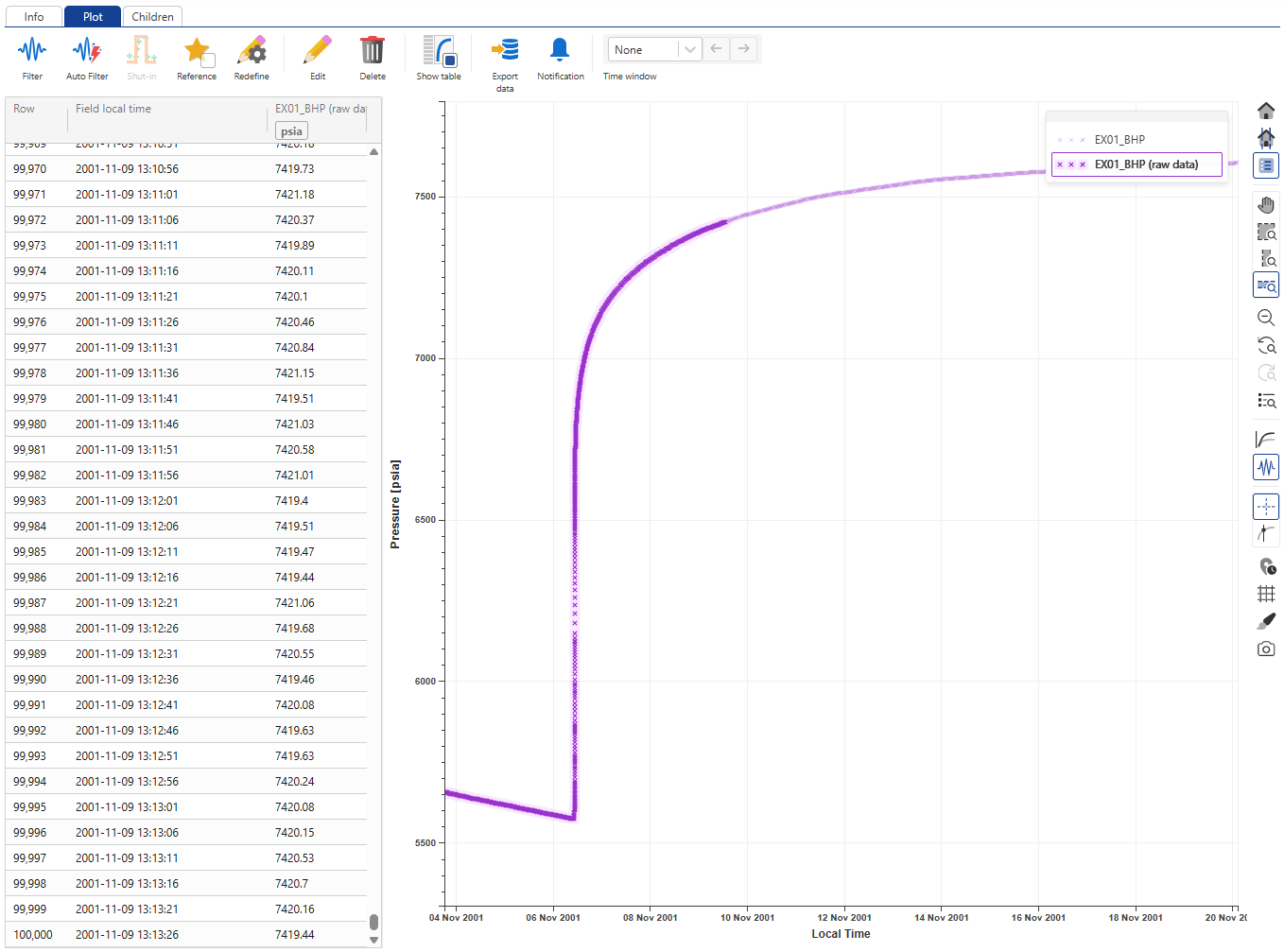
Select EX01_BHP in the field hierarchy:
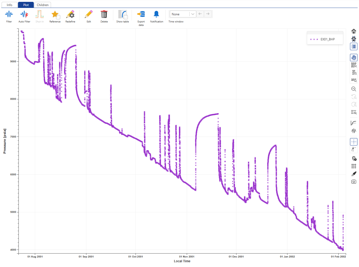 |
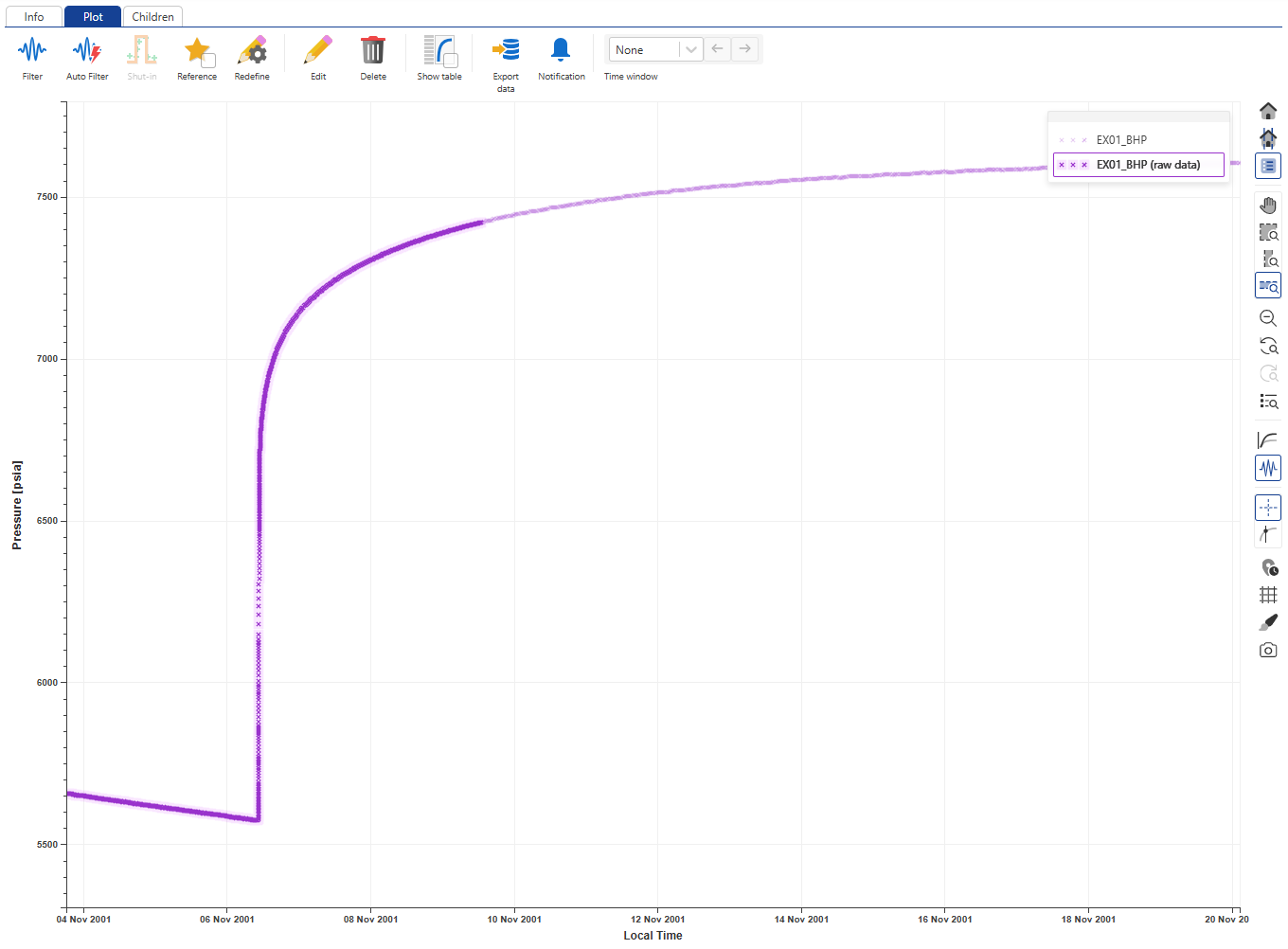
Zoom around area of interest and enable Raw data slice,  , in the toolbar to the right of the plot. The plot is updated and 100'000 points of the raw gauge data are highlighted on the plot starting from the left side of the window.
 |
To see the data values, click on Show table, .
.
 |
It is possible to zoom in/out of the plot or move an existing selection window on the data. As soon as the highlighted raw data slice is not adopted by the window, KA starts processing the gauge to show another slice of 100,000 points of the raw data.
Once done, click on  and
and  to the right of the plot to restore the view.
Filtering High Frequency Gauges
In KAPPA-Automate only high frequency data loaded as a gauge can undergo filtering.
In this section, we will create two different filters (and a third in the next section), with the same denoising but different decimation settings.
Setting up Filter #1
To setup a filtered data, select the gauge and under the Info or Plot tabs, click on Filter among the options listed at the top:
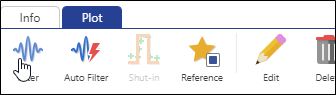 |
The Y Min, Y Max parameters can be used to exclude outliers from the data. X min is set to the Time of first point by default but may be changed by the user. Rename the filtered gauge to EX01_BHP_F:
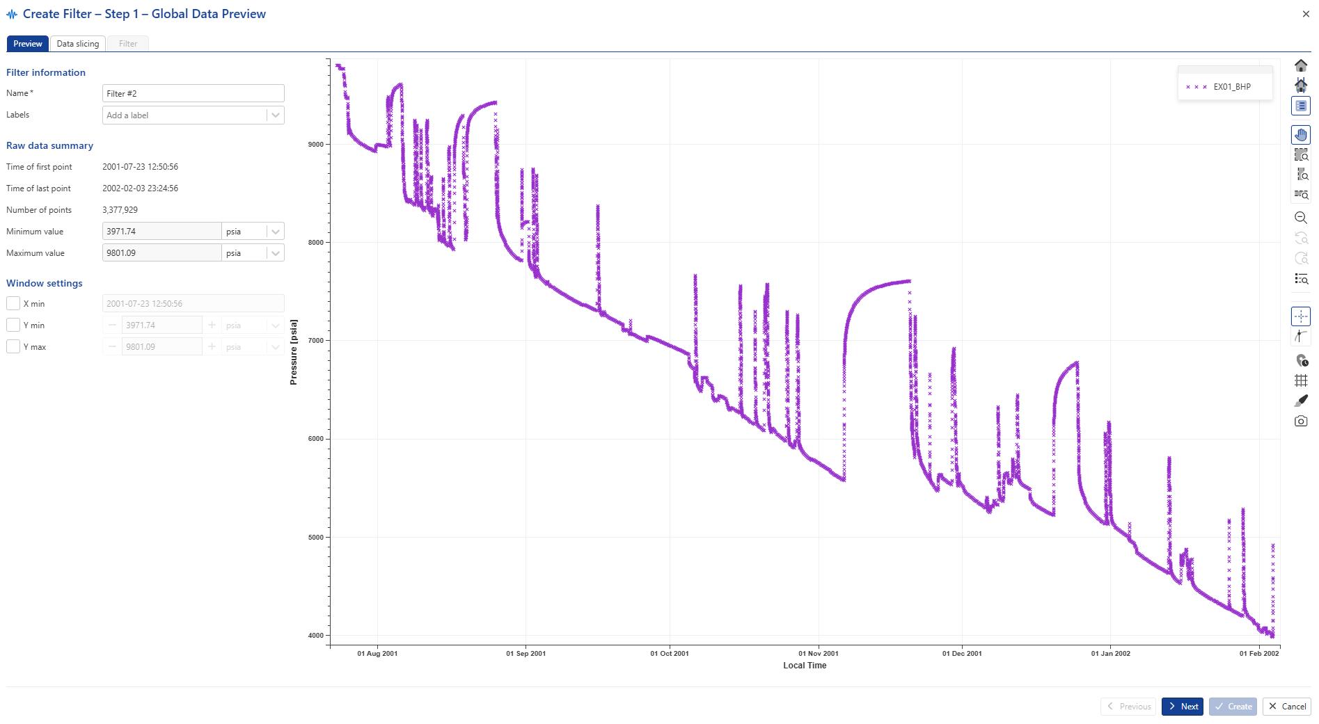 |
Keep the default values and click on Next to navigate to the Data slicing tab. The Data slicing tab shows a preview of the complete gauge in small plot on the left. The red vertical line marks the start of the data slice. The date and time are displayed in the Time of first point field under the Slice settings panel. The end of the data slice is controlled by the Size of slice parameter. Data points in the slice are shown on the large plot to the right. This plot shows all the raw data points in the slice.
Moving either the red vertical line in the full gauge preview or by inputting a date in the Time of first point, set the start of the slicing window to around 9th August 2001:
 |
The idea is to select a representative slice that can be used to set the filtering parameters. Participants may use a different slice if they wish.
Click on Next.
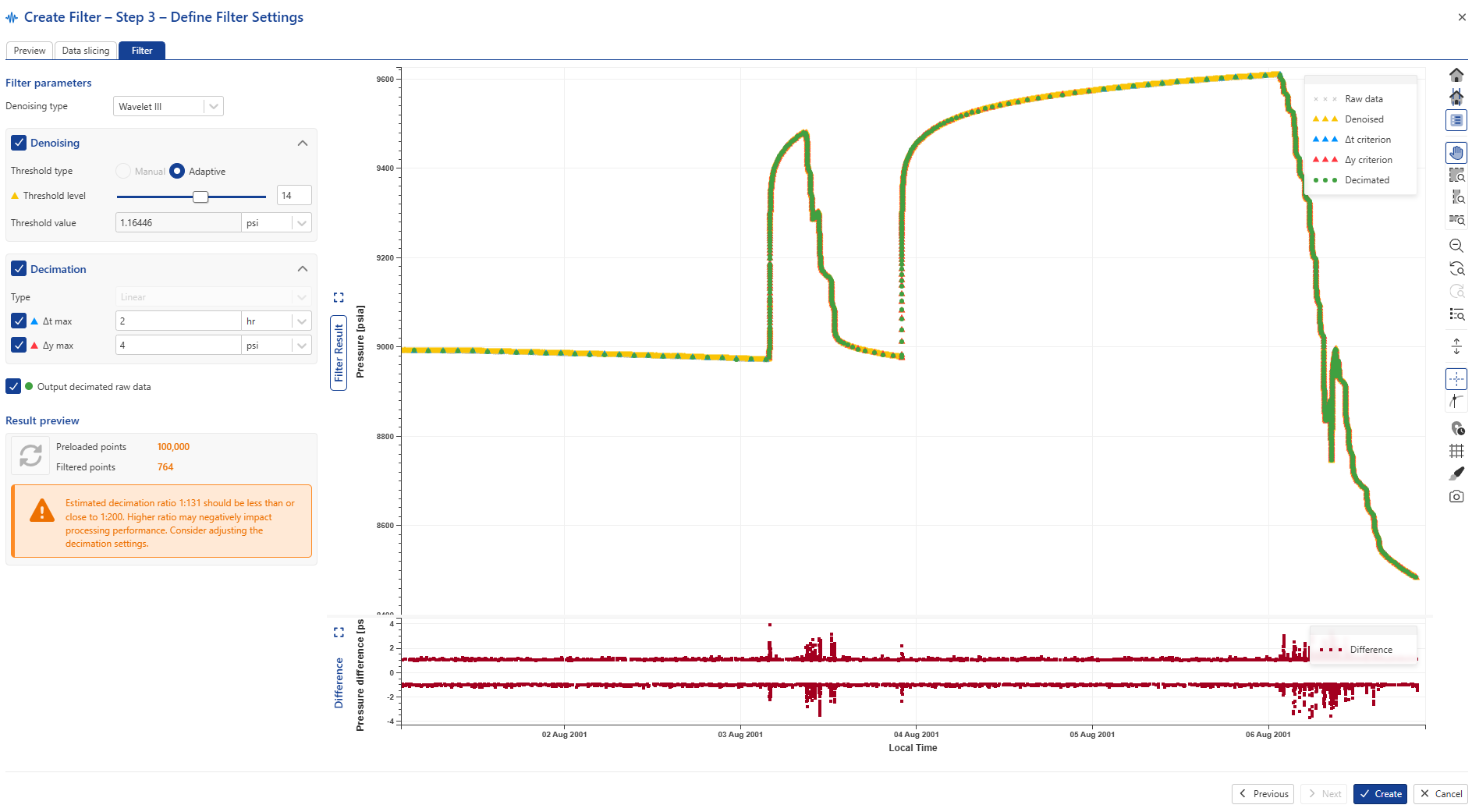
The first step in setting filtering parameters is to select appropriate Denoising parameters.
In the Filter tab keep the default Wavelet II setting and deselect Decimation. Next click on  and inspect the denoising results on the plot with zoom options.
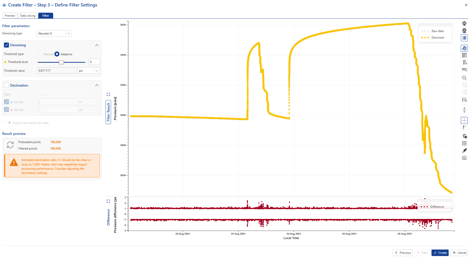 |
Raw data points are represented in grey, while the denoised data in yellow.
Use the Threshold level to adjust denoising level (set to 14 in the image below).
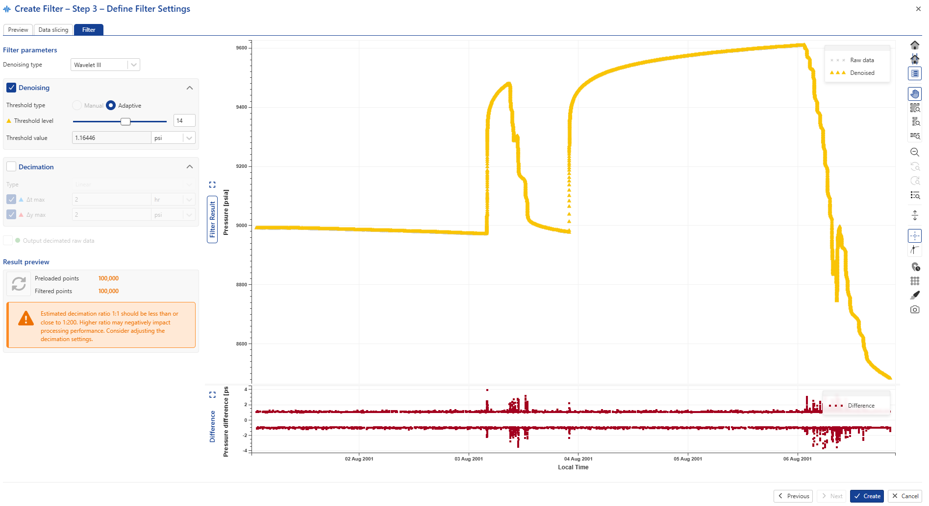 |
After an appropriate denoising level is selected switch Decimation on and click on to update the plot:
 |
Set the required decimation delta t and delta y criteria (2 hrs and 4 psia in the image below) and click on to visually inspect the results:
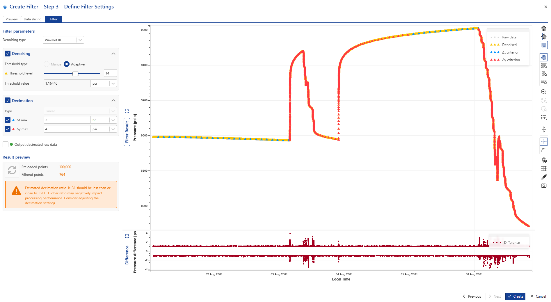 |
The data reduction from decimation can be viewed under the Results preview section:
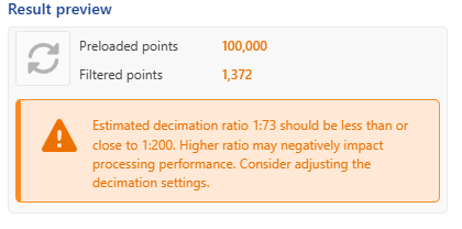 |
Use the Zoom in/out to inspect the decimation in other parts of the slice:
 |
Click on Create to accept the filter settings.
The filter will be listed under the parent gauge in the field hierarchy:
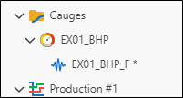 |
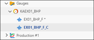
Setting up Filter #2
Repeat the same procedure as above, with the following changes:
Filter name: EX01_BHP_F_C
Decimation: Δt max = 24 hrs; Δy max = 1000 psia
Auto-Filter
An Auto-Filter bypasses the UI and creates a filter at once, using default settings.
Select EX01_BHP node and click on Auto-Filter,  . Rename the filtered data under EX01_BHP_F_AUTO:
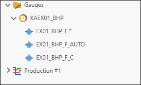 |
Loading Rate data
When a well is created, a Production node is automatically created under it. A single production node can carry all three phases. Multiple production nodes can be created for a given well.
 |
Select the Production #1 node in the field hierarchy and click on Gauge among the options listed at the top.
Repeat the same procedure as for the high frequency pressure gauge and select to load KAEX01q.kbl in the Tag list .
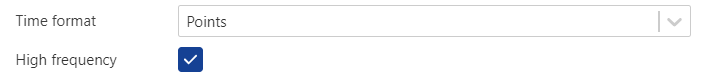
Change the gauge Name to EX01_qo and the Time format to Points. Check High frequency:
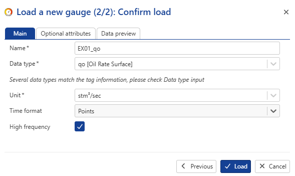 |
Click on Load. The oil node will be ‘filled’ under the production node:
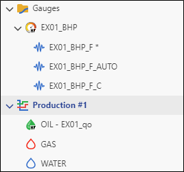 |
We will not load gas or water rate for this exercise.
Filtering High Frequency Rate Data
The high frequency rate data must also be filtered before proceeding. An Auto-Filter will be used for this purpose. This bypasses the UI and creates a filter at once, using default settings.
Select OIL – EX01_qo node and click on Auto-Filter, . Rename the filtered data under OIL – EX01_qo to EX01_qo_F:
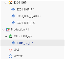 |
Shut-in Identification
Shut-in identification in KAPPA Automate follows the same principle as KAPPA Server. It can be performed on pressure (or temperature) history data. Shut-ins are identified by searching for discontinuities in the pressure data. Identified shut-ins are recorded in a special SIID logical channel that has the value of “1” for the duration of the shut-in and “0” everywhere else.
Only one Shut-in channel can be created for a well.
Select EX01_BHP_F in the field hierarchy. Under the info or Plot tabs, click on Shut-in ,  ,among the options listed at the top:
 |
In the consequent wizard, set Minimum shut-in duration to 24 hrs and Minimum pressure change to 1000 psi. Check Required validation:
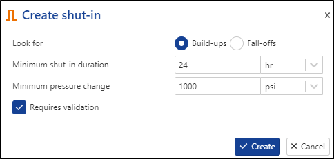 |
Click on Create.
Once done, a Shut-in node is added under the well node, with a child Raw Shut-in node:
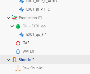 |
Shut-in Validation
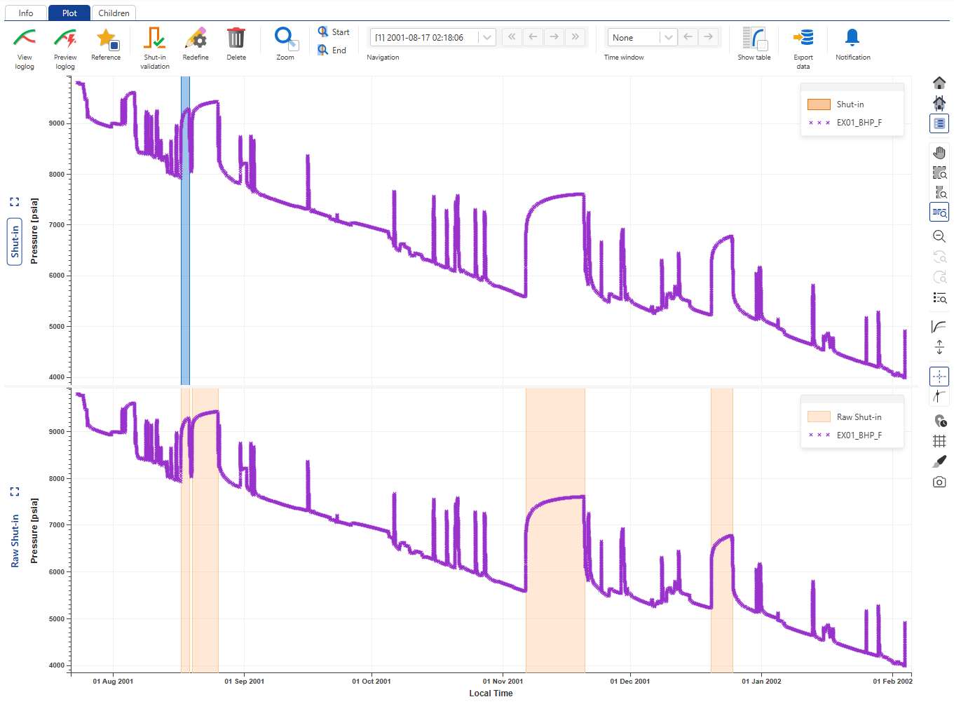
Click on the Shut-in node in the well hierarchy. Under the Plot tab, two plots are shown:
Shut-in plot: showing the pressure gauge used to identify shut-ins along with any validated shut-ins. At this stage, no shut-in is validated, so the plot only shows the pressure gauge.
Raw Shut-in plot: showing the pressure gauge used to identify shut-ins along with any raw shut-ins.
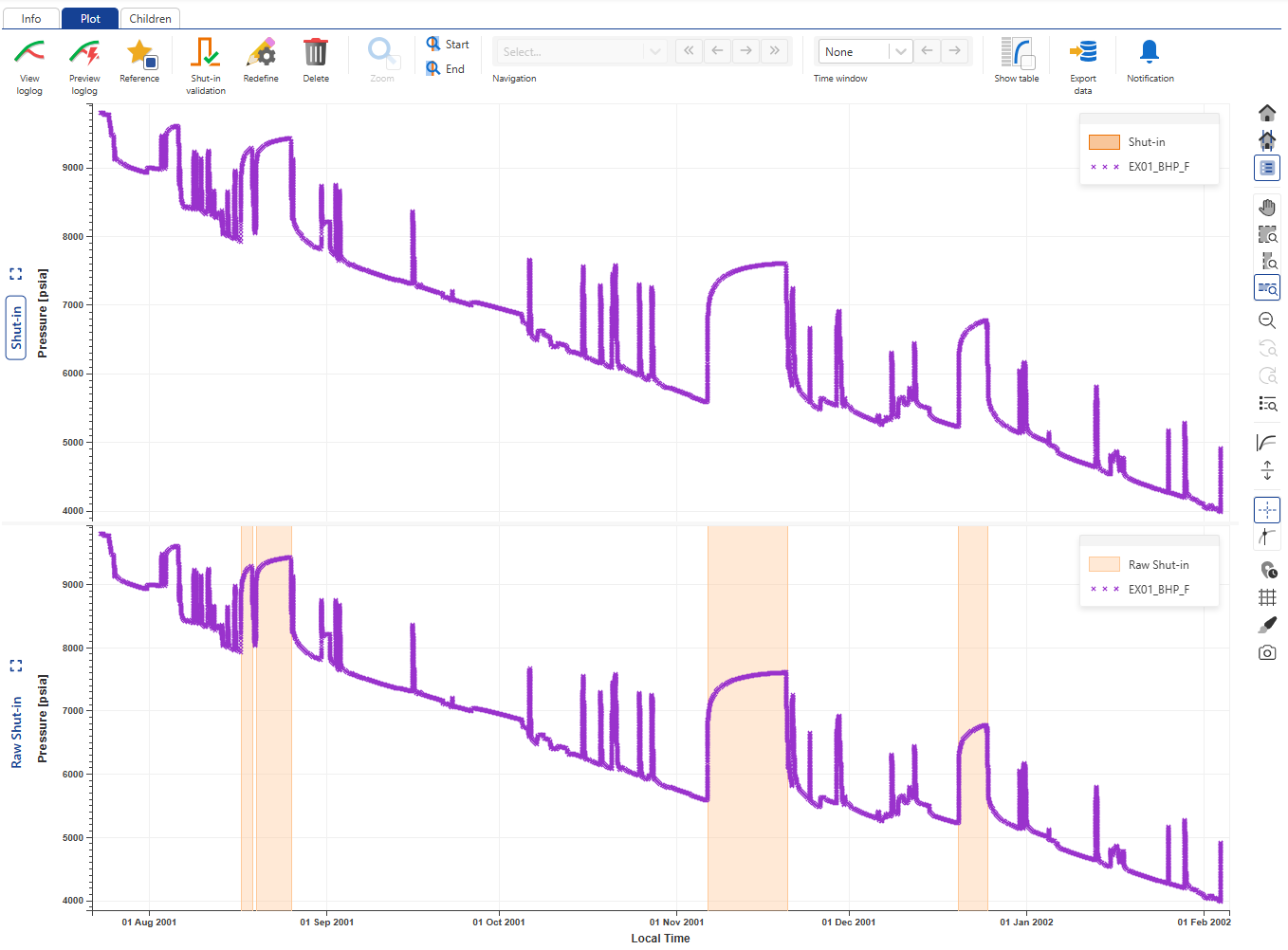 |
Copying Raw Shut-ins to Validated Shut-ins plot
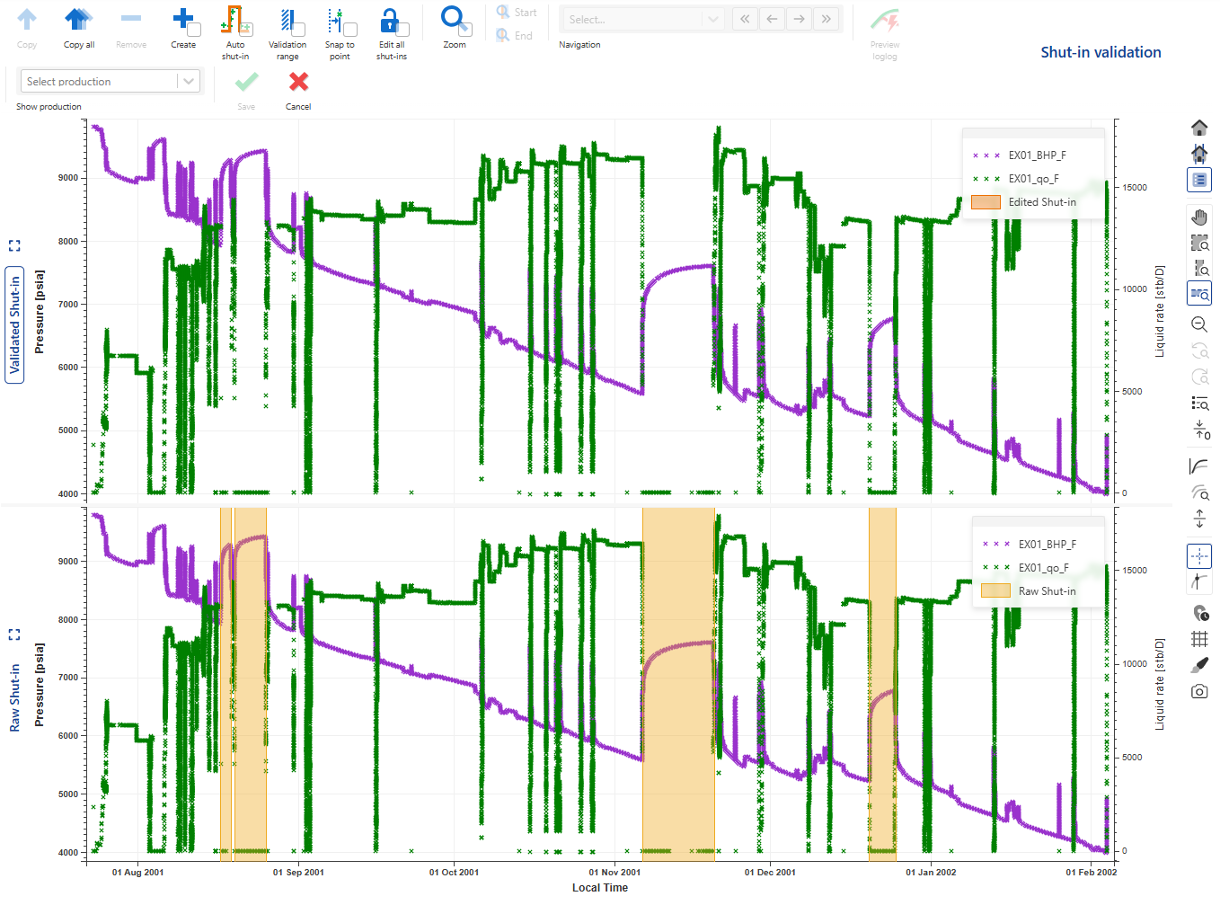
Click on Shut-in validation,  , among the options at the top, under the Info or Plot tab. In the Shut-in validation mode, the plot options at the top show the following:
 |
Two plots are shown:
Validated Shut-in plot: showing the pressure gauge used to identify shut-ins along with auxilary rate gauge and any shut-in copied over from the detected shut-in plot.
Detected Shut-in plot: showing the gauge used to identify shut-ins along with auxilary rate gauge and any detected shut-ins.
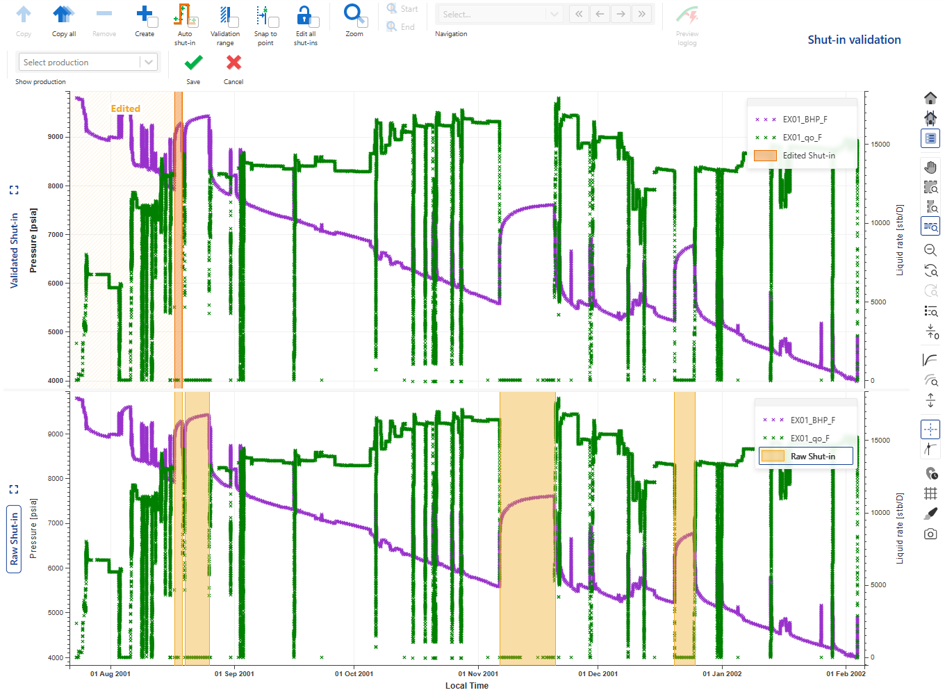
To mimic a realistic scenario, let’s imagine we only have data till the end of the first Shut-in. So, we will limit our validation to the first shut-in at this point.
Select the shut-in on the Detected Shut-in pane (click inside the highlighted area to select) and click on Copy to copy it to the Validated Shut-in pane (Alternatively, double click inside the highlighted area of the shut-in):
 |
QCing copied Shut-in
Once copied, the next step is to QC the shut-ins before validating them. Part of the QC could be to ensure the start and end of the Shut-in has been correctly identified.
Select a recently copied shut-in in the Validated Shut-in pane. This will turn the selected shut-in highlight to blue. Click on Zoom to zoom in on the selected shut-in. The vertical lines marking the start and end of the shut-in can now be interactively edited:
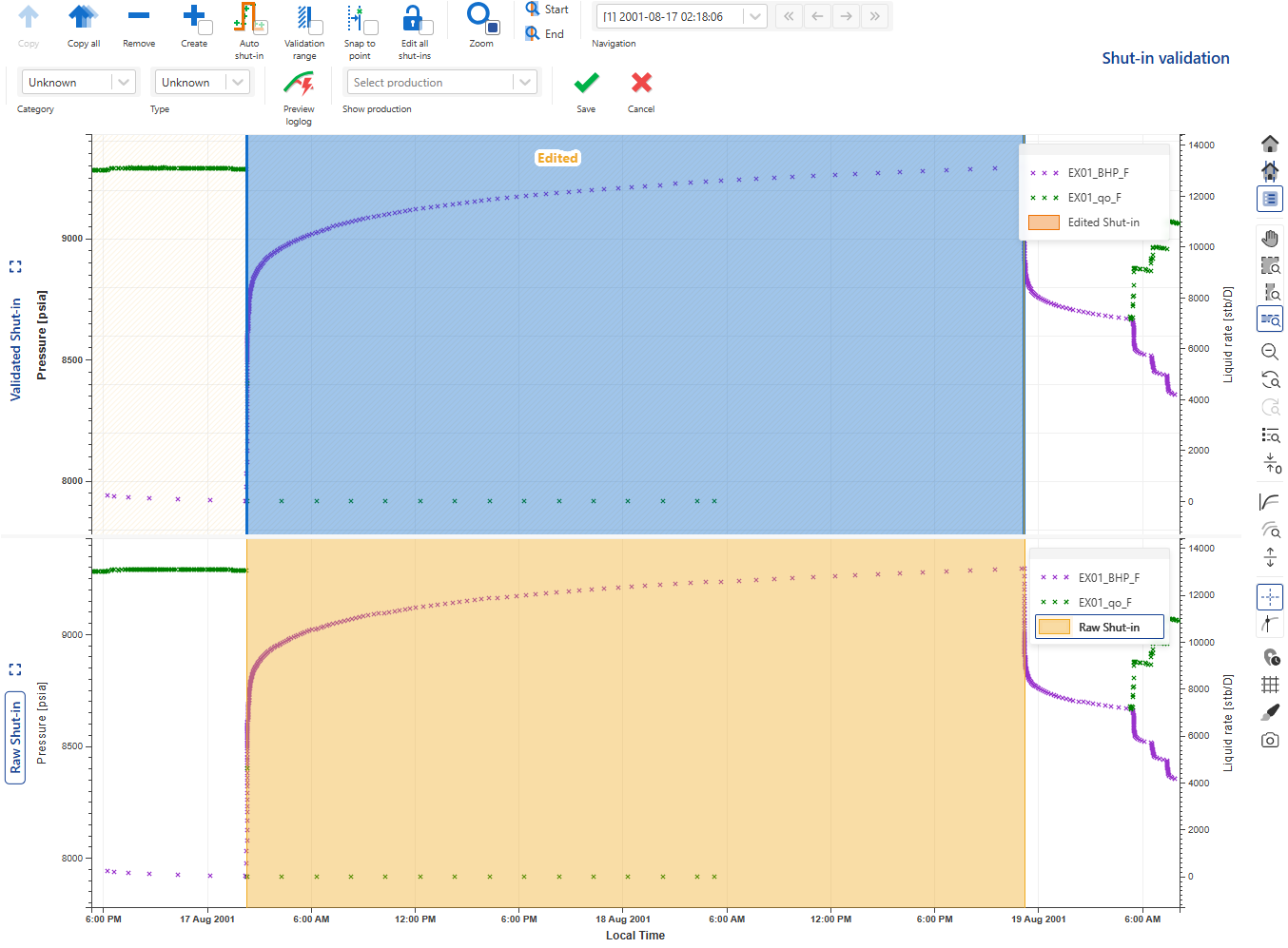 |
In this mode, the Navigation options become available which can be used to toggle between the unvalidated/recently copied shut-ins. No change is required at this stage as the detected start and end of the shut-in are satisfactory.
Before validating the SI, it is a good idea to preview the resulting loglog plot. Click on Preview loglog above the plot:
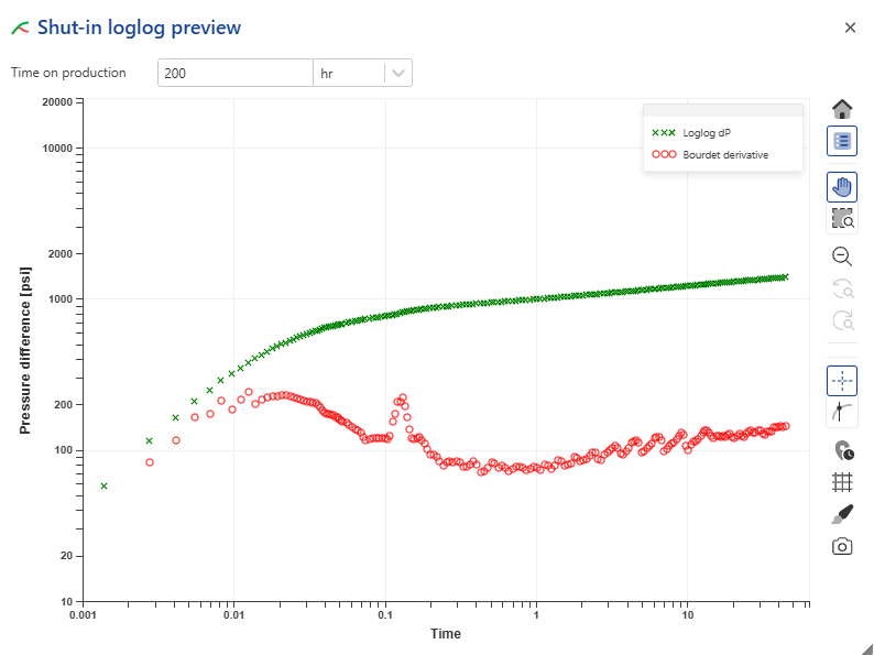 |
Note that the presence of a rate gauge (raw, filtered or corrected), although can be helpful, is not required for SIID. Therefore, this loglog plot only uses Horner superposition, where tp can be edited by the user (default: 200 hrs). All seems OK here. Close the preview form.
Validating the Shut-ins
Once the needed shut-ins have been copied and QC’ed, they can be validated by clicking on Save:
 |
Corrected Production
Once shut-ins have been validated, the logical Shut-in channel can be used to create a corrected production channel.
Click on the Filtered Production node and under the Info or Plot tab, click on Corrected Production:
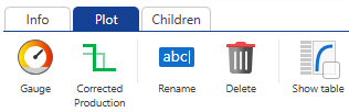 |
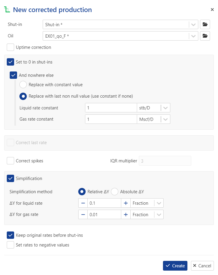
This launches the following wizard:
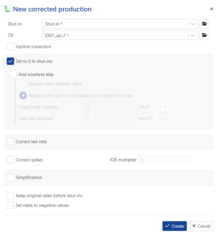
Set the following parameters:
Uptime correction: disabled
And nowhere else: enabled
Simplification: enabled
ΔY for liquid rate = 0.1
Keep original rates before shut-ins: enabled
A corrected production node is created in the field hierarchy under the well node:
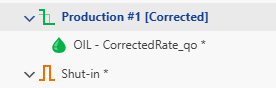 |
Viewing PTA Loglog Plot inside KA
Once the corrected production has been created, click on the Shut-in* node in the field hierarchy and under the Plot tab, click on View loglog,  , among the options at the top:
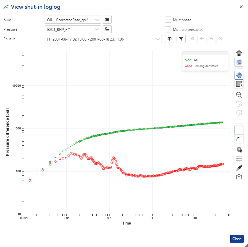 |
Note
In the background, KAPPA-Automate is calling the PTA µ-service, which creates a temporary Saphir document, extracts the shut-in and sends the loglog plot data back to KA to plot. µ-services will be discussed later during the training.
Creating User Plots
We will now create a few custom plots to better view what has been done so far.
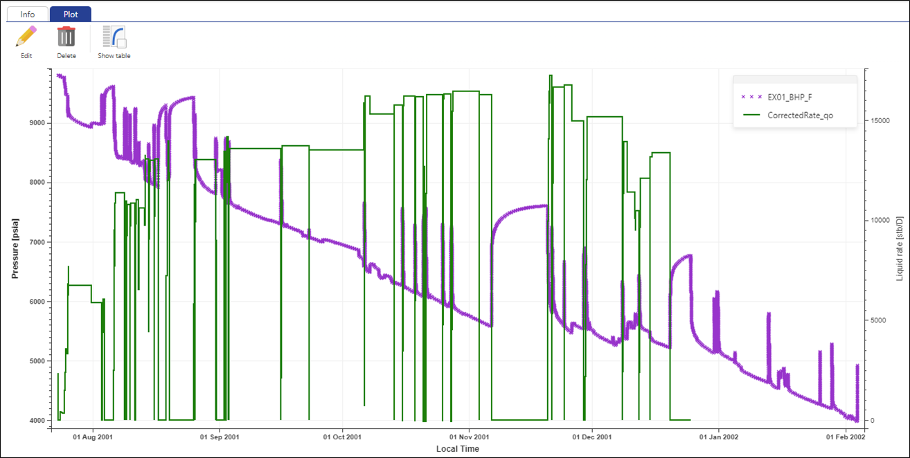
Select the well in the field hierarchy and under the Info tab, click on Plot,  , among the options at the top. Call the Plot Production Data and select EX01_BHP_F gauge and the corrected production nodes:
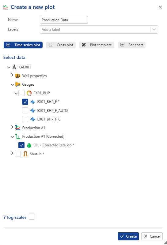 |
Click on Create.
The plot will be added under a newly created User plots folder in the field hierarchy:
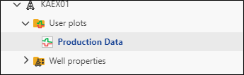 |
The plot shows that the rate data are synchronized with the pressure data. To inspect in detail, use the zoom in functions.
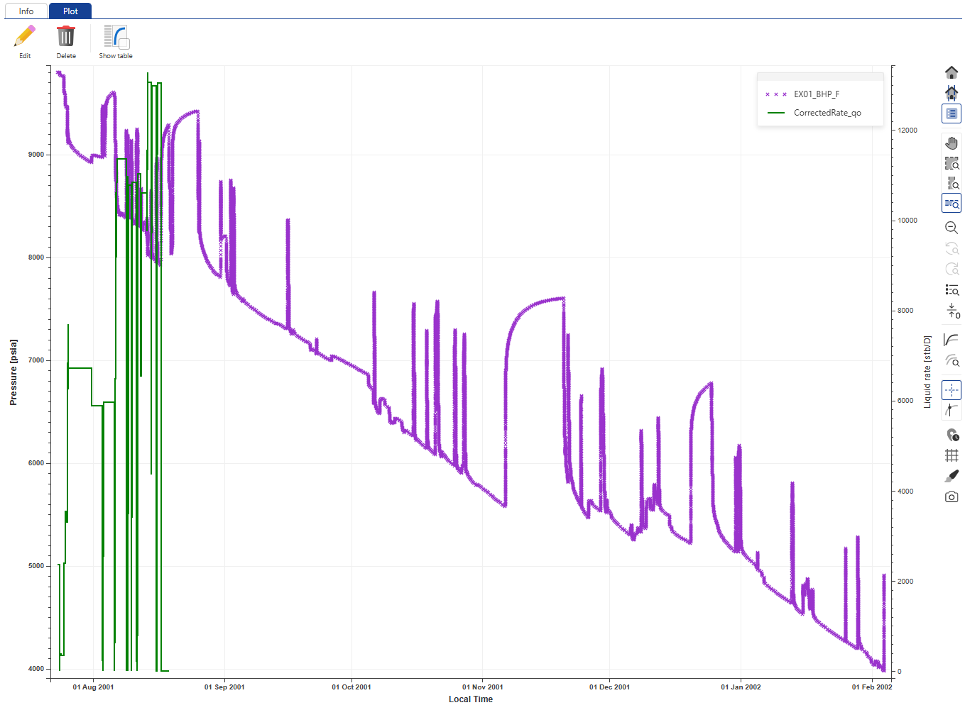 |
Proceed with creating another plot called Fine and Coarse Filters and select to display EX01_BHP_F and EX01_BHP_F_C on this plot:
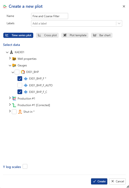 |
By default, both gauges have the same aspect, making it difficult to identify them.
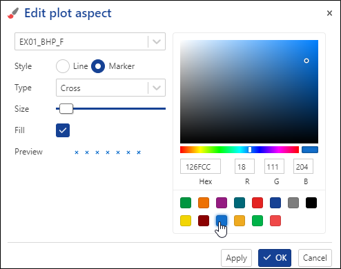
Click on Edit aspect, , in the plot options on the right. Change the color of EX01_BHP_F to blue:
Using the drop-down list, switch to EX01_BHP_F_C and change its color to orange, Type to circle and increase the size a little:
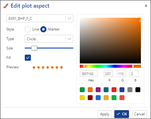 |
Click on OK:
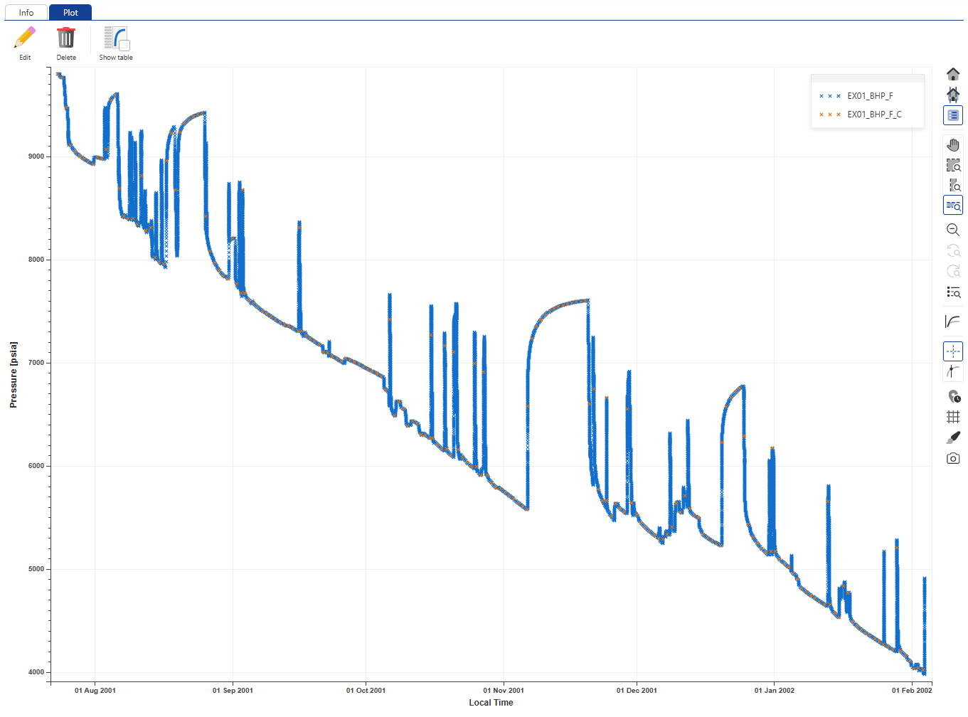 |
Opening a KA field in KW Browser
Select the field node in the KA hierarchy and under the Info tab, click on Open in KW,  , in the options at the top:
 |
This will launch KAPPA-Workstation 5.50.xx with the KW Browser open. The field will be listed in the browser:
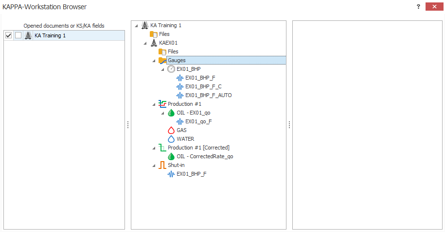 |
Gauges of interest shall be sent to Saphir through a Drag ‘n’ Drop (DnD) via the KW Browser. For this, the target Saphir (or Topaze, Rubis etc.) file must first be created/opened in KW.
Create a new PTA document
Create a new Saphir file.
Set the Reference time of the document equal to the Min X value in the pressure gauge:
 |
Proceed with document creation.
Save this document somewhere on disc and call it iPTA Start.
Transfer gauges to KW
In KW Browser, select the KA field on one side and the Saphir document on the other. Expand the field hierarchy to the BHP_LF and corrected production channels. Expand the Saphir document to well data.
Drag and drop EX01_BHP_F to the Pressures node and OIL – CorrectedRate_qo to Productions node under Saphir well data:
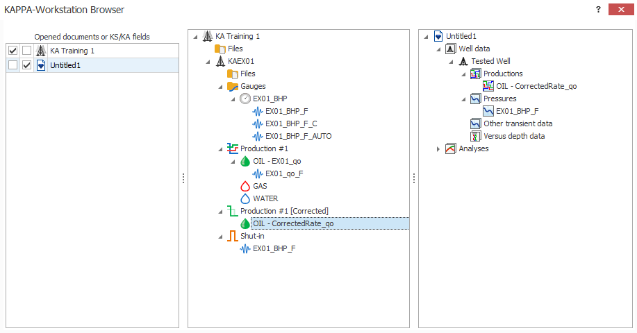 |
Since the gauge EX01_BHP_F was loaded all the way to the end, go to Edit P, select the pressure data after the end of production history and delete it. This is to mimic what one might get in a real production environment.
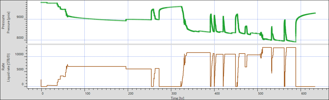 |
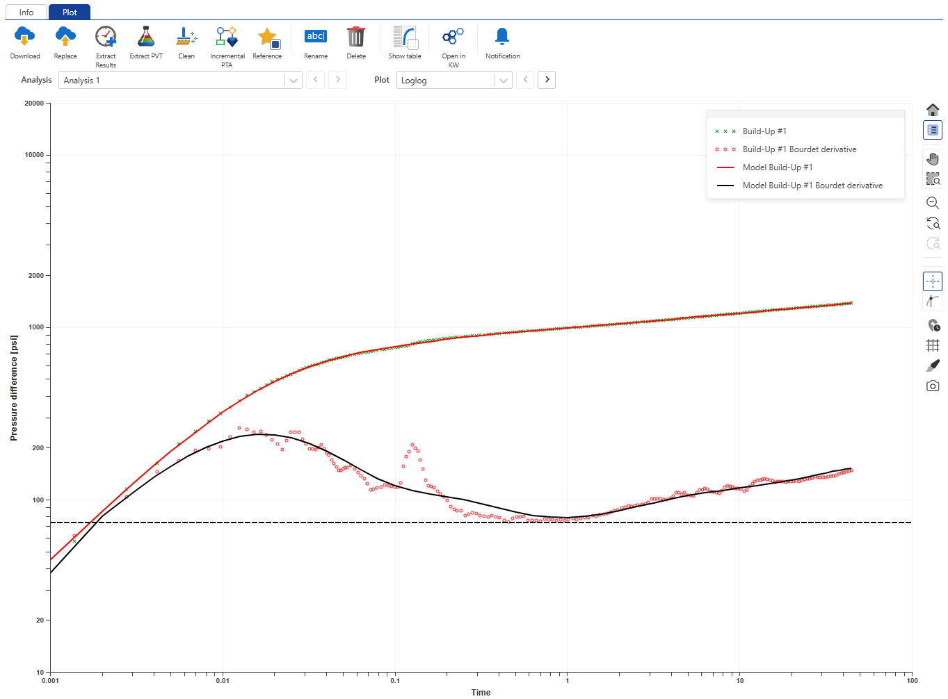
Extraction + Model in KW
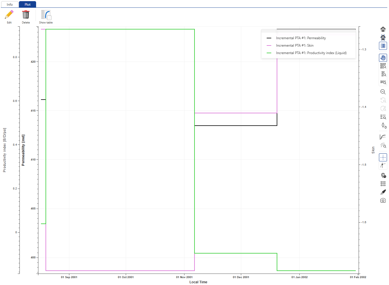
Extract the BU data. Set analysis tools to changing wellbore storage and rectangular boundary. Match the tools to data on the loglog plot:
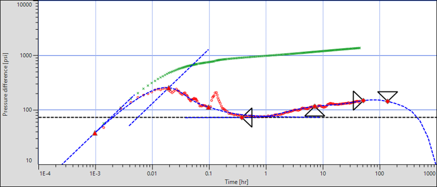 |
Generate auto-analytical model (Shift + Analytical), followed by Improve to obtain a decent match:
 |
Save the file. Call it EX01_iPTA_Start.
Create a new RTA document
Repeat the same process with Topaze with one exception:
Drag the ‘EX01_BHP_F_C’ pressure gauge.
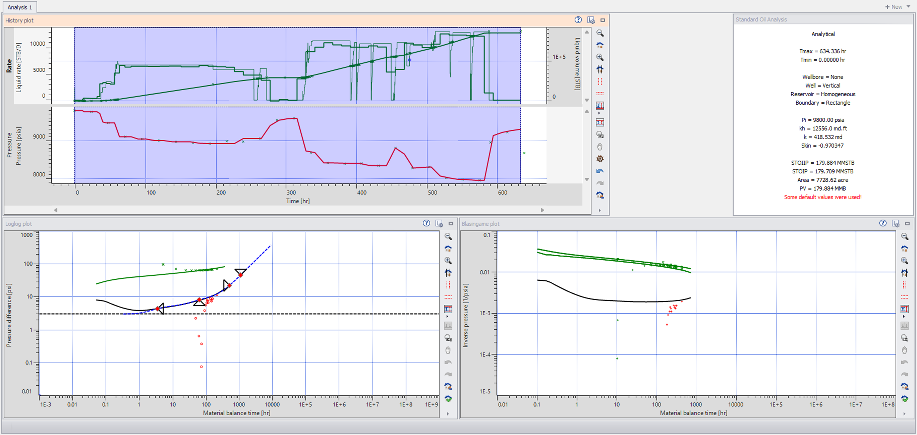 |
Run a forecast in Topaze with the following settings:
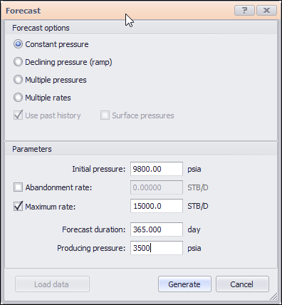 |
To get something like this:
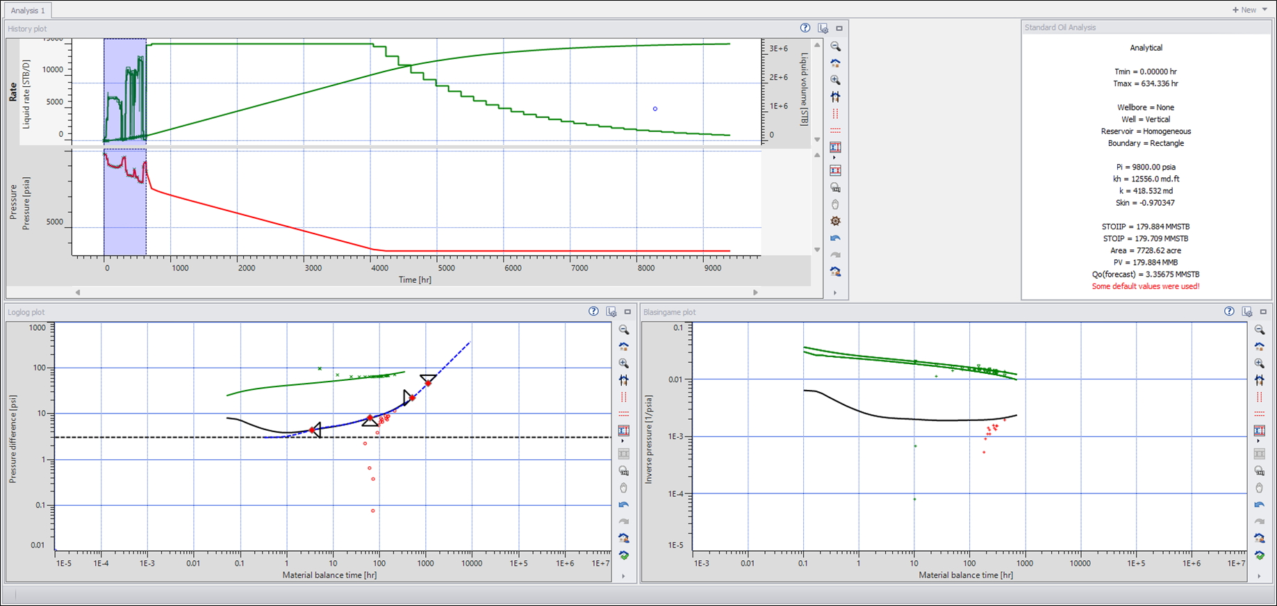 |
Save the file and EX01_iRTA_Start.kt5.
Upload KW file to KA
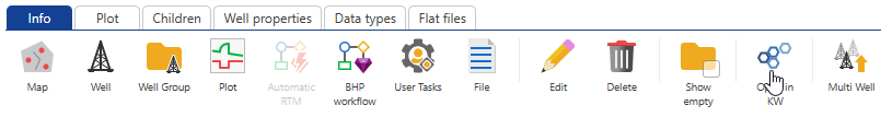
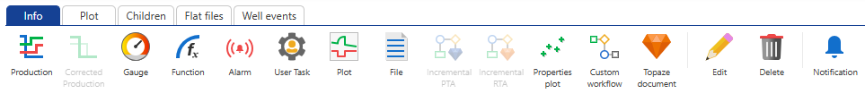
When loading for the first time, select the well in the field hierarchy and click on File,  , under the Info tab:
 |
Select the files and click on Open. A new Files folder will be created under the well where the files will be stored:
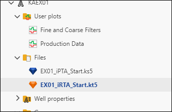 |
Additional files may be loaded using the steps described above. Alternatively, click on the Files folder and use the File option under the Info tab.
It is possible to view in the K-A client the document information and results as well as the main plots.
Content Visualization
When Saphir or Topaze documents are uploaded under a well or field they are automatically pre-processed by KAPPA-Automate. The following are extracted as part of document pre-processing:
Analyses results: To view analyses results, click on the file in the document hierarchy, go to the Info tab and scroll down to the table under the KAPPA results section.
Analysis plots: To view analyses plots, click on the file in the document hierarchy and go to the Plot tab. Users can toggle through the different analyses in the file as well as the plots in each. The following plots are available to view:
Saphir: Loglog plot, History plot and Semilog plot
Topaze: Loglog plot and History plot
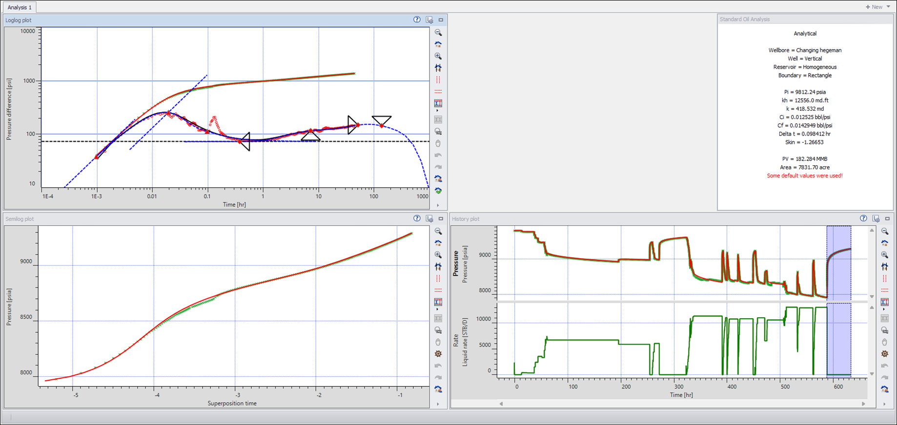
Select the EX01_iPTA_Start.ks5 file in the field hierarchy. By Default, the loglog plot from the Saphir file will be shown:
 |
Using the Plot dropdown menu, select History plot:
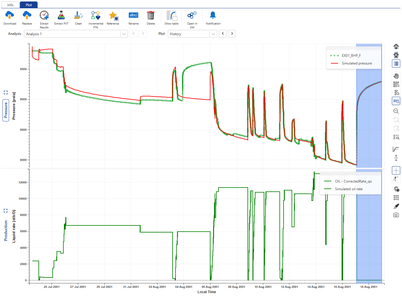 |
Switch to the Info tab and scroll down to view the analysis results:
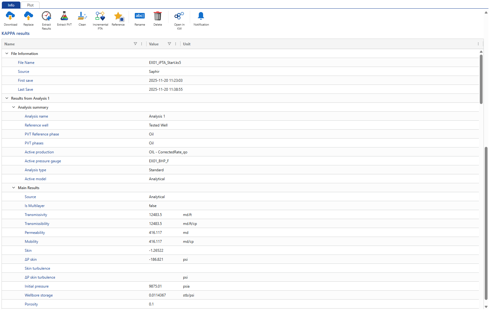 |
Result extraction into well properties
Analysis results can be extracted from the documents stored under a well and saved as well properties, the main use case being to track the evolution of parameters with time. Well properties results can be plotted or used in further processes or computations. Extraction of results can be configured as desired from the XML file contained in the K-W archives. It can be triggered on an individual document, or a folder. Finally, one can extract results from valid analyses only or all of them. Some workflows that create K-W documents automatically also trigger results extraction – this is the case with iPTA or iRTA described next.
Click on Extract Results,  , among the options at the top:
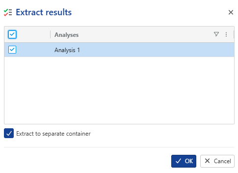 |
Select Analysis 1, check the option Extract to separate container, then click OK. This will create a new well properties container using the same file name:
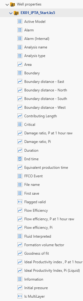 |
Inside the EX01_iPTA_Start.ks5 container, click on Permeability and switch to the Plot tab:
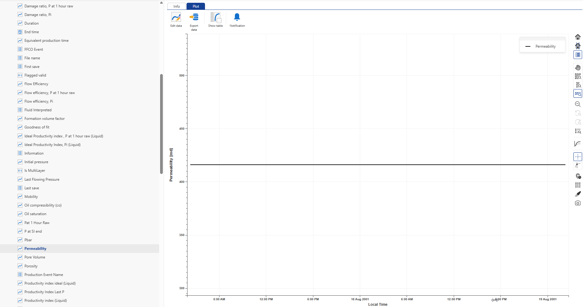 |
Since this is the first extraction for this well, only a single value from the analysis is displayed. View other well properties in the same manner.
Prerequisites
To start an iPTA workflow, the following pre-requisites must be met:
A Saphir file must be uploaded under the well. This file will serve as the seed document for iPTA.
A Shut-in channel mut exist for the well.
A corrected production must exist for the well.
Launching iPTA
To launch iPTA workflow, select a Saphir file (EX01_iPTA_Start.ks5) in the field hierarchy and click on Incremental PTA, , under the Info or Plot tab:
 |
This will launch the following iPTA wizard:
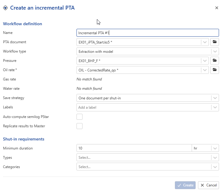 |
Name: this is a required field. Users can give whatever name they wish. For this session, let’s keep the default
PTA document: This is the seed document for iPTA. Model parameters will be picked up from this Saphir file. Since the iPTA was called after selecting the Saphir file, iPTA_Start.ks5 is already selected. Leave the selection as is.
Pressure: The pressure gauge to use for iPTA. Leave the default selection (EX01_BHP_F)
Corrected production: Leave the default selection (OIL – CorrectedRate_qo)
Defining iPTA Strategy
Save Strategy
There are two ways users can create/update Saphir files with new data:
Single document with one analysis per shut-in: any new data are sent to the PTA document defined in the iPTA creation wizard and a new analysis is created for each shut-in. A maximum of 10 analyses can be created in a single document, after which a new document will automatically be created.
One document per shut-in: Each shut-in is extracted in a new document. Data in each document are truncated at the extracted shut-in.
For this session, select the latter option.
Workflow type
There are three types of iPTA workflows available:
Extraction only: This is the only available option if the selected PTA document does not contain a model. The data up to a given shut-in will be sent to the PTA µ-service which will perform the extraction.
Extraction with model: In addition to the steps explained in (1) above, the model in the PTA document is extended up to the shut-in being processed.
Extraction with model + improve: In addition to the steps explained in (2) above, if this option is selected, an improve strategy is requested by the user at the time of iPTA creation. The user can specify what model parameters to improve on, as well as their ranges. During execution, after the model has been extended to the processed shut-in, in improve on the loglog plot is performed.
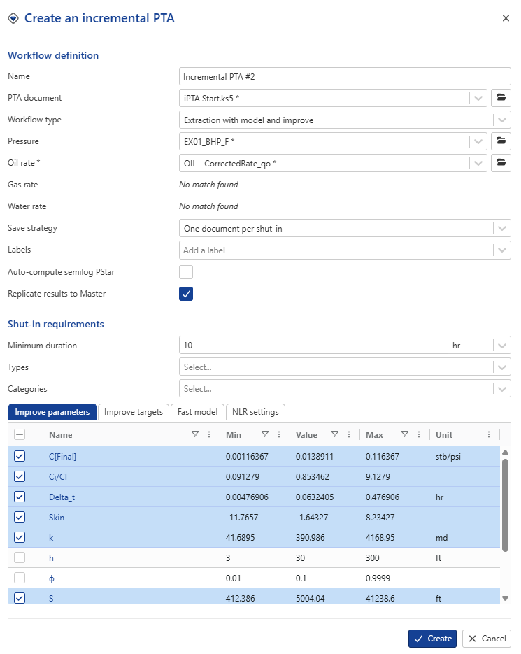
For this session, select the third option.
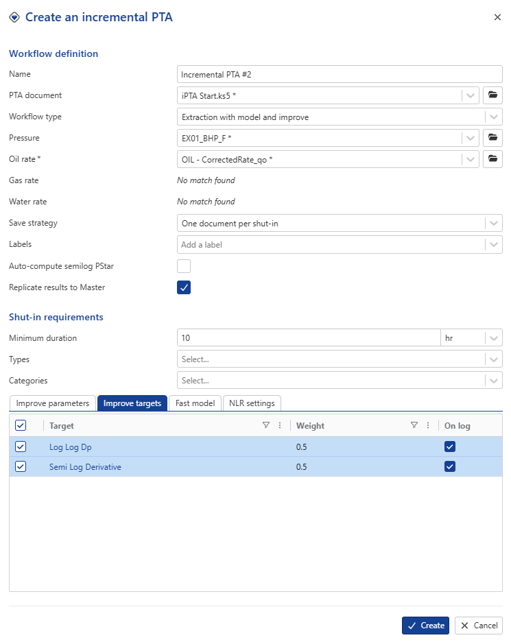
In the Improve parameters tab, select to improve on model: C[Final], Ci/Cf, Delta_t, Skin, k and boundaries (S, N, W, E). Select Replicate results to Master.
In Improve target tab, set the objective function to a 50/50 wight between Log-Log Δp and Semi-Log Derivative, and check the option On log.
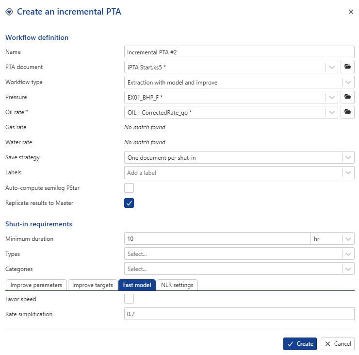
In the Fast model tab, leave it unchecked, as we will not use it for this example.
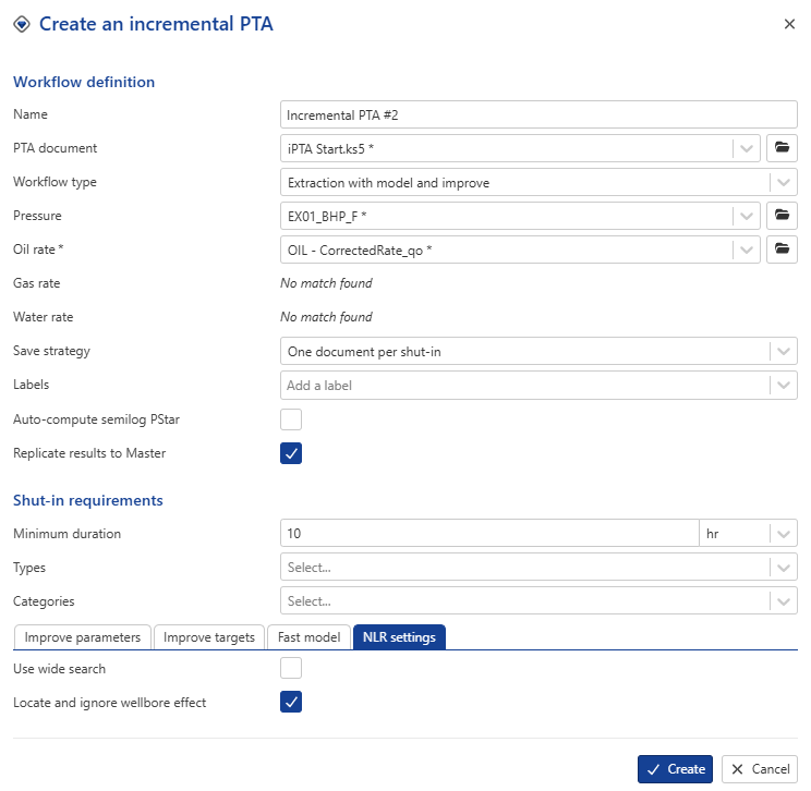
In NLR settings tab, check Locate and ignore wellbore effect. This option automatically removes the wellbore storage portion from the objective function, provided the algorithm successfully detects the end of the wellbore storage period.
 |
 |
 |
 |
Click on Create.
Viewing iPTA results
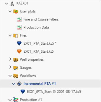
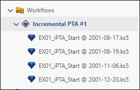
When an iPTA is first launched, it will create a new container under Well properties node in the field hierarchy, named Incremental PTA #1. A new folder called Workflows will also be created in the field hierarchy, with the iPTA and any files created by this iPTA listed there:
 |
iPTA Results under Workflows
Since the Single document with one analysis per shut-in save strategy was selected, one document, created under the Incremental PTA #1 (or whatever name was given to the iPTA) node. The document name follows this logic: <<Seed file name>> - <<start @ shut-in date>>
So far, we only have one validated SI for this well. Therefore, only a single file is shown, showing the same model as the seed file.
iPTA Results under Well properties
The contents under the Incremental PTA #1 container are like those under the Master container. They will automatically be updated/appended as new shut-ins are processed, giving users a complete time-lapsed view of the different well properties. Create a new User Plot under the well and call it PI, k S. Select Productivity Index, Permeability and Skin under Master container:
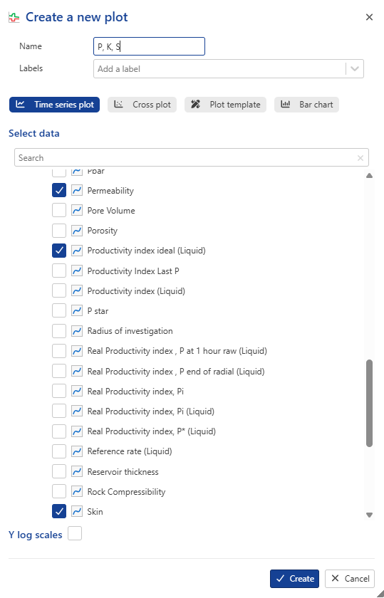 |
Click on Create:
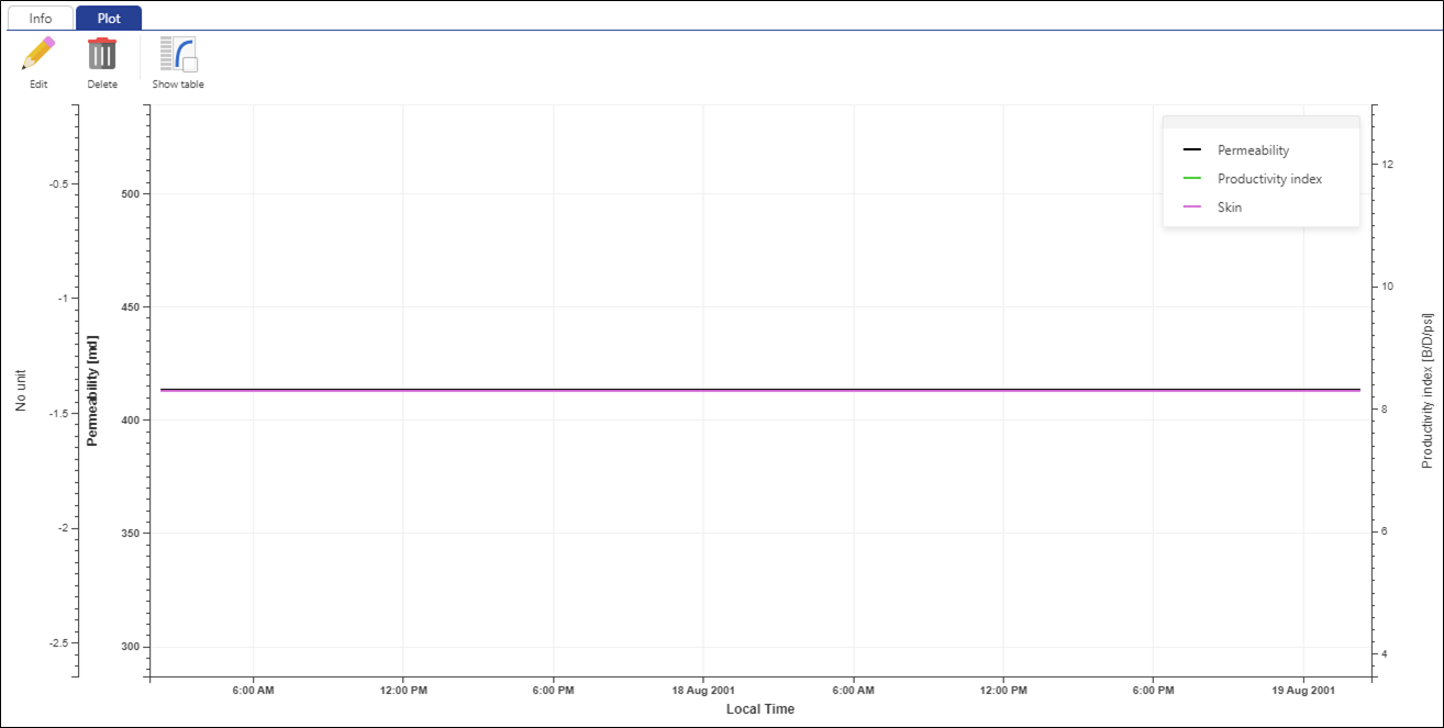 |
While the iPTA was set up, we had assumed only one (or few) existing SIs. Let us now simulate more data being mirrored into KA: how the iPTA reacts in the background to data increments.
The trigger to any operation related to PTA is identification of a new shut-in. To mimic this, let us now go back to shut-in validation and validate additional shut-ins.
Click on Shut-in in the field hierarchy and click on Shut-in validation, , among the options at the top. Click on Copy all, , to copy all the detected shut-ins to the Validated Shut-in pane:
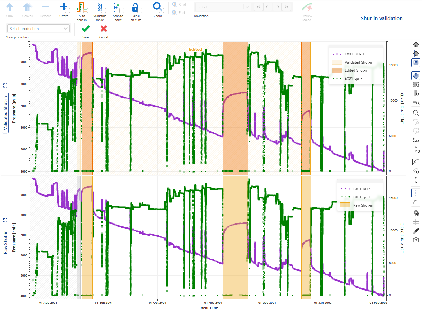 |
Using the Zoom, Previous and Next options above the plot, navigate through the different shut-ins to QC their start and end times. Once done, click on Save, .
.
This will trigger an update of all what we set up in this session:
Corrected production channel will be updated.
The new shut-ins will be extracted.
Data will be sent to Saphir.
The model will be regenerated on the new shut-in.
To improve match on the loglog plot, improve will run on WBS, k, and S.
The new Saphir document will be added to the Incremental PTA #1 node under Workflows.
Select any file under this node, go to plot tab and compare the loglog match for the different shut-ins:
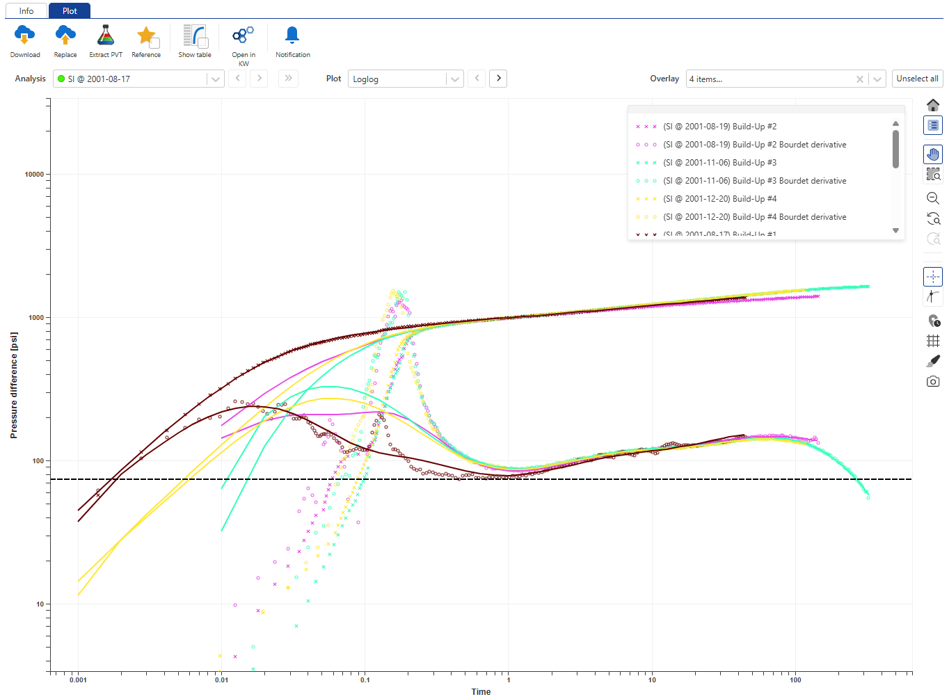
Container for Incremental PTA #1 under Well properties will be updated. Since Replicate to Master was checked, the master well properties container will also be updated.
Any custom user task will run and update its own results.
The User plots will be updated as the new data are available. Select the PI, k, S user plot to see the evolution of these parameters with time:
The speed at which all this happens depends on the infrastructure and resources available for the different processes.
Introduction
A gauge is typically a mirror of a tag in a data source (historian or database). A gauge is typed precisely; and for instance, a particular pressure time series could be loaded as simply Pressure or more strongly typed as Bottom-hole pressure, Casing pressure etc. This is what we did when loading the pressure gauge. Typing is important as it will help automated processes select the proper input. When there are several instances of the same data type, it is possible to flag one as the reference. Once again this will guide automatic selection.
Labels can be added without restrictions to hierarchical objects. This is yet another way of enabling automatic selection later.
Adding labels to data
Select EX01_BHP_F and go to the Info tab. In the Custom labels field, enter finefilter and validate with Enter. Similarly, add the following labels to the other two filtered data:
EX01_BHP_F_C: coarsefilter
EX01_BHP_F_AUTO: autofilter
Note that the data type for all these filters is BHP.
Go to the Incremental RTA #1 container and select Simulated pressure. Notice its data type is Pressure.
Creating functions
Go to the automation section. We will define a simple function which adds 1000 psia to a pressure gauge. We will use data typing and labelling to allow automatic selection of the gauge to use.
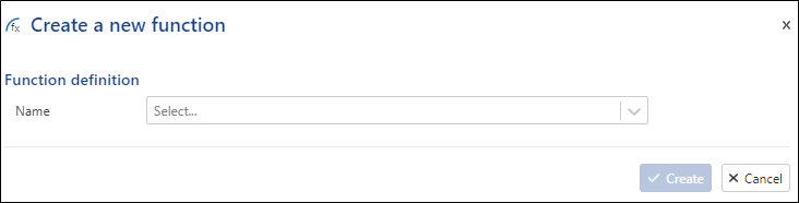
Under the Functions page, click on Create:
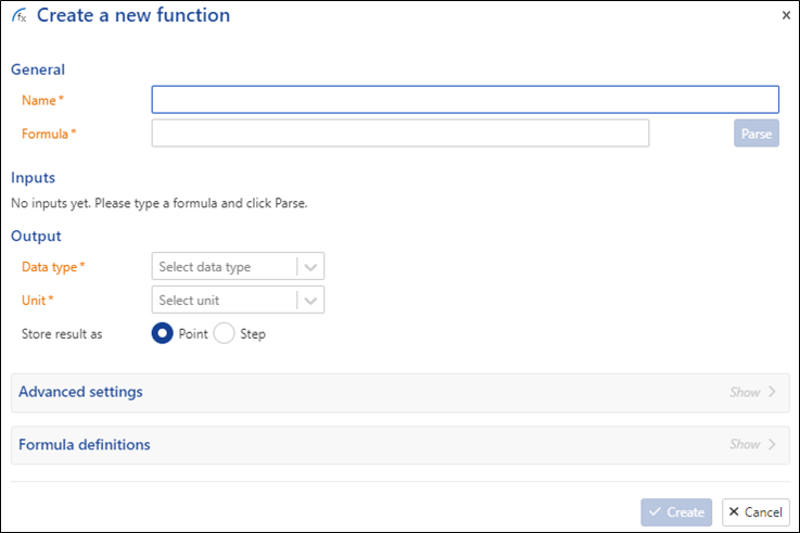 |
Call the function P + 1000 (Pressure)
Type the following for the formula: P + 1000
Click on Parse:
In the Inputs section, set the data type to BHP [Bottom-hole Pressure] and units to psia.
In the Output section, set the data type to BHP [Bottom-hole Pressure] and units to psia:
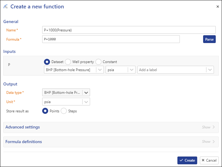
Click on Create.
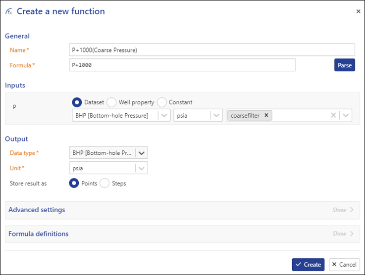
Create a new function, with the same Formula but the following differences:
Name: P + 1000 (Coarse Pressure)
Inputs: Data Type: BHP [Bottom-hole Pressure]
Inputs: Label: coarsefilter
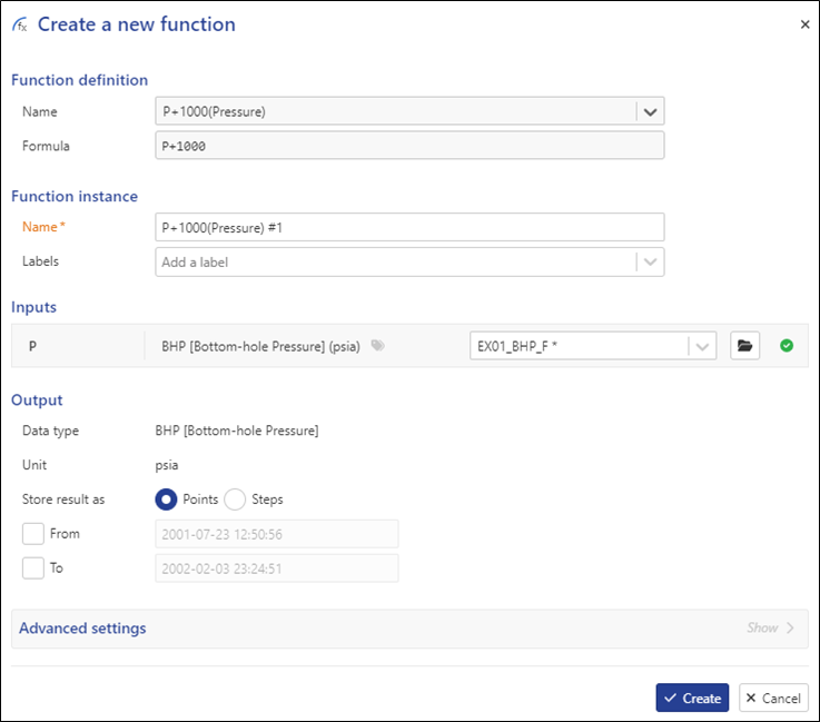
Creating function instances
Go back to the field and select the KAEX01 well node.
Click on Function among the options in the ribbon at the top:
 |
From the drop-down list, select P + 1000 (Pressure):
|
Based on the data type defined when creating the function, all BHP gauges under the well are listed (the reference one being the default selection):
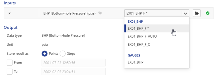 |
Switch to EX01_BHP_F_C and click on Create to create the function instance. Create another function and this time select P + 1000 (Coarse Pressure):
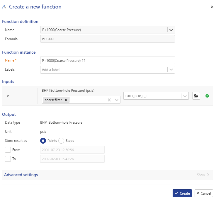 |
The correct pressure gauge based on data type + label is automatically selected. Once done, the two outputs may be compared with the original/input data using custom plots.
Introduction
Plot templates can be created at the global K-A level, at the Field, Well Group and Well level. These provide a default view of the data at the selected level in the heirarchy. Plot templates benefit for data typing and labeling, which offer a flexible way to customize data display/visualization.
Applying/Editing template at field level
Select field node and go to the Plot tab.
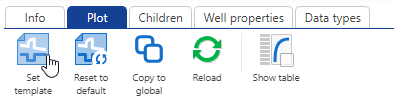 |
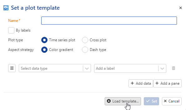
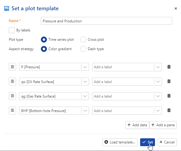
Click on Set template, . This will open the definition plot template instance applied to the field.
Click on Load template
 |
Select Pressure and production which represents the default template
 |
Press Ok:
 |
Now we see the pressure gauges in addition to the rate gauges.
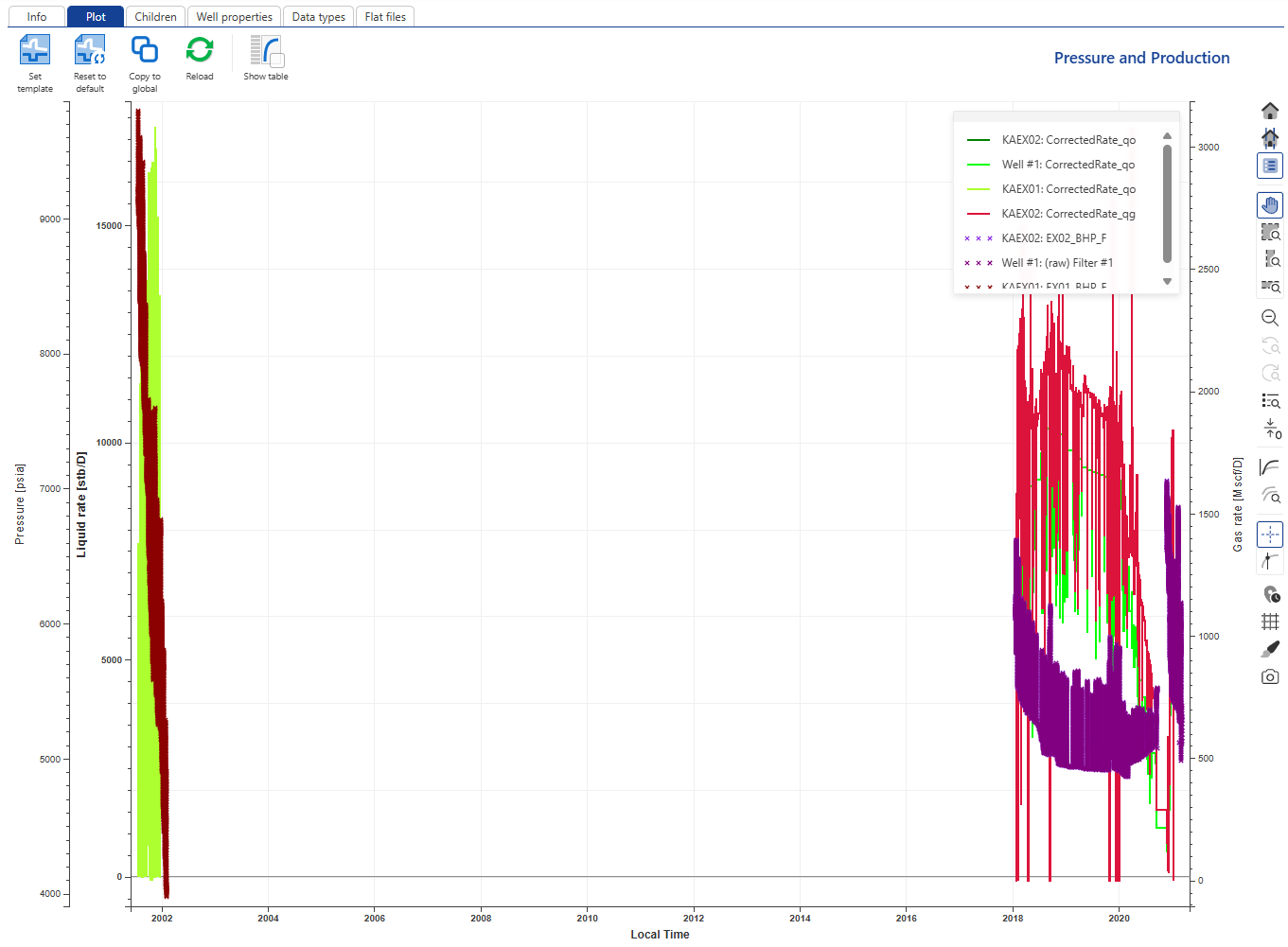 |
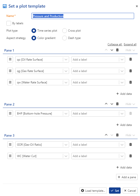
Let us make the field level plot a little clearer. Click on Set template, . Click on Add a pane and in Pane 2, select BHP. Remove BHP from Pane 1.
Add a new pane and select to display GOR and WC in the third pane.
Add a fourth pane with the SI channel.
Note
All these changes are applied to the instance of the plot template. The original template definition is not affected and it is possible to reset back to it if needed by clicking on Reset default template , .
.
Applying/Editing template at Well level
Select KAEX01 well in the field heirarcy and click on Set template, . Keep BHP in pane 1. Add a new pane and add oil rate, GOR and WC. Add a third pane.
Click on  and select well property.
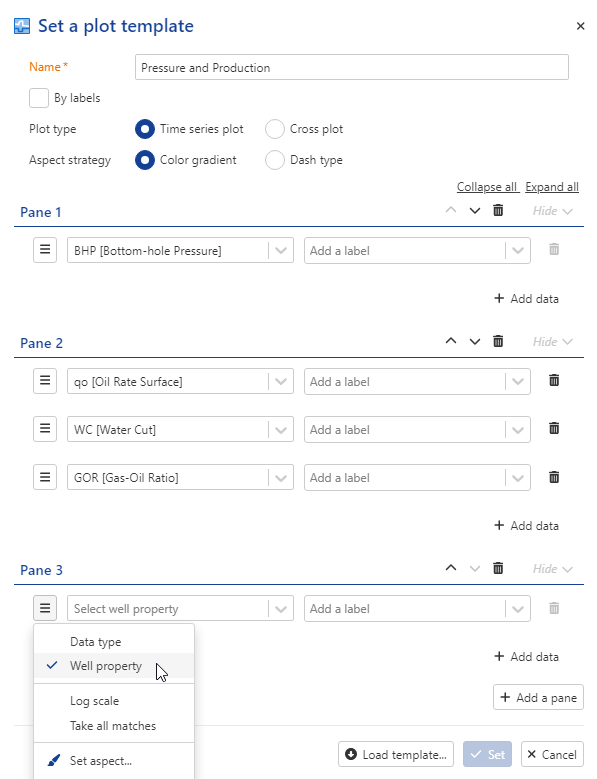
Add permeability
Repeat the steps to add skin:
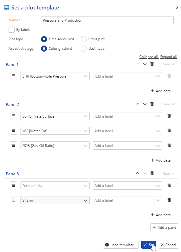
Press Set