Simplified RTA (sRTA)
Objectives
The sRTA user task provides an implementation of the workflow described in URTeC 5096 (Acuna, 2021), namely:
Automatic RTA diagnostic and determination of:
# of zones (1 or 2)
Half-fractional dimension(s)
mQ
Skin term (“b”)
Wellbore storage term (“c”)
Xmf(s)
Initialization of simplified RTA model from diagnostic results
User-specified uncertainty (ranges)
User-specified uncertainty (ranges)
Input
This section describes the required and optional input to run the sRTA user task. The input comes in many forms, including Topaze files, well properties, and direct input into the user task UI.
Prerequisites
Before creating the user task for the well to be modeled, the engineer must first define the PVT for the sRTA model as well as several properties for the well.
PVT: The PVT is defined via a Topaze file, which must be uploaded to either the field or the well. The PVT is used to calculate the total rate for the well and the total compressibility of the system. The PVT types can be volatile oil, condensate, dead oil, and dry gas (all which can optionally include water). Constant values of Bo, Bg, Bw, Rs, and rs are extracted from the PVT description to calculate the total rate. In addition, in the case of gas wells, the Topaze file is used by the RTA micro-service to calculate the pseudo-pressures which are used by the simplified RTA model.
Well properties: A certain number of well properties must be defined, which are described in the table below. The well property is identified by the alias in the user task code. The property name is what is visible in the property table and is used only for display purposes, hence configurable. Note that the properties representing the reservoir thickness, permeability, porosity and initial pressure are pre-existing properties. The other properties in the list below do not exist by default and hence must be created manually in Well properties catalog (Automation Mode).
Alias | Name | Description | Measure |
|---|---|---|---|
WellLength | Well length | The completion length of the well | Length |
MainResults_Porosity | Porosity | The porosity of the reservoir | No unit |
MainResults_Permeability | Permeability | The permeability of the reservoir | Permeability |
StageOrClusterSpacing | Stage/cluster spacing | The property is used to initialize the SRV radius (rSRV) | Length |
ModelBoundary_ReservoirThickness | Thickness | The thickness of the reservoir | Length |
BoundaryType | Boundary type | Choices are "Infinite", "Side well", "Inner well", or "SRV only". | No unit (string) |
WellSpacing | Well spacing | This property is used to initialize the SRV width (WSRV). If the boundary type is “Infinite”, then this property is optional. | Length |
MainResults_InitialPressure | Initial pressure | (Optional). When available, the pressure drop for the well will be calculated using this value. Otherwise, the pressure drop is calculated by taking the maximum value in the history as the initial pressure. | Pressure |
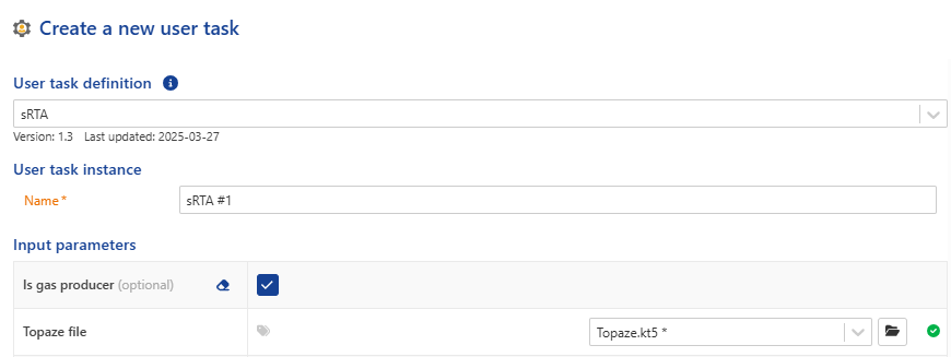
Inputs
The user task UI has a large number of inputs, which are described below. The various inputs are placed into different categories for better understanding.
General: There are several general inputs which are required, described in the table below.
Name | Description |
|---|---|
Is gas producer | If checked (true), the well is considered as a gas producer (dry gas or condensate). Used to configure the type of output (barrels of oil equivalent or Mcf equivalent). |
Topaze file | As described above, the Topaze file contains the PVT description of the field or well. |
Wait time for relaunching forecast | The user task will be rerun when the accumulated amount of data exceeds this time. Default is 60 days. |
Starting date | (Optional). The user may wish to modify the start date of the production. This may be desirable when the initial stage of production is followed by a long shut-in period. |


General input
Datasets: Certain datasets are required, depending on the main phase (PVT). A brief description is given in the table below.
Input name | Description | Data type |
|---|---|---|
Pressure data type | Specifies the data type of the pressure (BHP or P) | Enumerated values |
Pressure | Required. Assumed to be low frequency data (daily pressures, for example) | Pressure (either BHP or P). Low frequency point data |
OilRate | Required if the PVT description is dead oil, volatile oil or condensate gas. | Oil rate (qo), step data |
WaterRate | Optional for all PVT descriptions. | Water rate (qo), step data |
GasRate | Required of the PVT description is dry gas, condensate gas, or volatile oil | Gas rate (qg), step data |


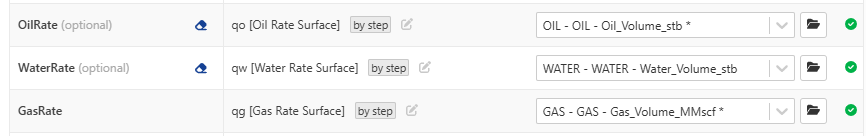
Input datasets
Uncertainty definition: One or more of the well or reservoir properties must be specified as uncertain to run the probabilistic forecasts. The main input (and dependent input) is described in the table below. The “Dependent Input” column describes input which depends on preceding input value in the table.
Input name | Dependent Input | Description |
|---|---|---|
Is porosity uncertain | If selected, the porosity is considered uncertain and is allowed to vary within the defined range. | |
Porosity (+/-) | Defines the upper and lower bounds of the porosity around the base value specified by the well property. The minimum porosity is a small, positive number. | |
Is permeability uncertain | If selected, the permeability is considered uncertain and is allowed to vary within the defined range. | |
Permeability (+/- Orders of magnitude) | Defines the upper and lower bounds (in orders of magnitude) around the base value specified by the well property. | |
Is SRV radius uncertain | If selected, the SRV radius (rSRV) is considered uncertain and is allowed to vary within the defined range. In the case where two zones are detected, this value pertains to the first (inner) zone. | |
SRV radius (+/-) | Defines the upper and lower bounds of rSRV around the value determined by the diagnostic. The minimum rSRV is equal to 1. | |
Is Xmf uncertain | If selected, the Xmf is considered uncertain and is allowed to vary within the defined range. In the case where two zones are detected, this value pertains to the first (inner) zone. | |
Xmf (+/- Orders of magnitude) | Defines the upper and lower bounds (in terms of orders of magnitude) of Xmf around the value as determined by the diagnostic. | |
Is thickness uncertain | If selected, the reservoir thickness (in terms of contributing to production) is treated as uncertain | |
Thickness (Min) | The minimum value of the thickness. | |
Thickness (Max) | The maximum value of the thickness | |
Is skin uncertain | If selected, the skin is considered uncertain and is allowed to vary within the defined range. | |
Skin (+/-) | Defines the upper and lower bounds around the skin value determined by the diagnostic. | |
Is fractional half-dimension uncertain | If selected, the fractional half-dimension is considered uncertain and is allowed to vary within the defined range. In the case of two zones, this pertains to the first (inner) zone | |
Fractional half-dimension (+/-) | Defines the upper and lower bounds around the fractional half-dimension determined by the diagnostic. |
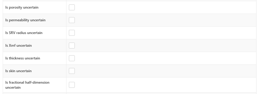
Uncertainty definition (no uncertainty)
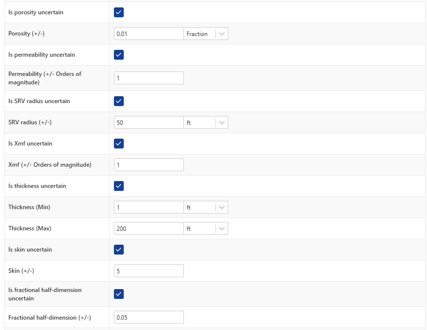
Uncertainty definition
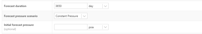
Forecast: There are two main inputs for defining the forecast period and pressure evolution. There will be one pressure value per week of forecast. By default, the constant pressure for the forecast (and first pressure in pressure decline scenario) is calculated as the median value of the last week of pressure data during the historical period.
Input name | Dependent Input | Description |
|---|---|---|
Initial forecast pressure | (Optional). The user can specify an alternative initial forecast pressure value using this input. | |
Forecast duration | The duration of the forecast. | |
Forecast pressure scenario | Describes the evolution of the pressure in the forecast. Choices are “Pressure Decline” and “Constant Pressure”. | |
Pressure decline gradient (pressure/year) | The decline of the pressure per year of forecast. Only visible if the “Pressure Decline” scenario is selected. | |
Minimum forecast pressure | The minimum pressure in the forecast period. Only visible if the “Pressure Decline” scenario is selected. |
Forecast input
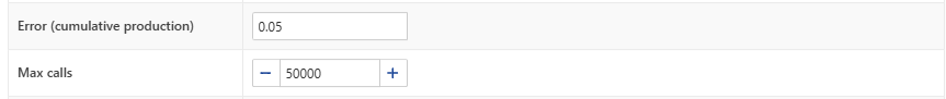
Sampling: The probabilistic forecasts are derived using Nested Sampling (NS). The “Max calls” input the time of the sampling and hence the approximation of the posterior. Note that if this is set to a large number, the user task may time out unless the time-out duration is increased.
Input name | Description |
|---|---|
Error (cumulative production) | This value determines the amount of error that the NS employs in the likelihood function (objective function). A higher value will allow for a greater spread in uncertainty during the historical period. A very low value will force the uncertainty band to be smaller, and increase the time for convergence to the posterior. |
Max calls | The maximum number of function evaluations performed to calculate the probabilistic forecasts. |
Sampling input
The input values may require tuning to obtain the desired results. See the output section below for more information.
Output
The sRTA user task outputs several datasets, including:
Total cumulative production (calculated from data)
Cumulative production phase ratios (GOR, WOR, WGR, CGR)
Pseudo-pressures (in the case of gas wells, derived from pressure values)
Forecast pressure employed in forecasts
Probabilistic forecast of total cumulative production and deduced rates from the NS algorithm (i.e. P1, P5, P10, P25, P50, P75, P90, P95, P99).
This is the direct output of the sRTA equations.
Phase cumulative production and rates, derived from the cumulative phase production ratios and the total cumulative production coming from the sRTA. Forecasts for cumulative phase production and rates assume a constant value of the cumulative phase ratios going into the future.
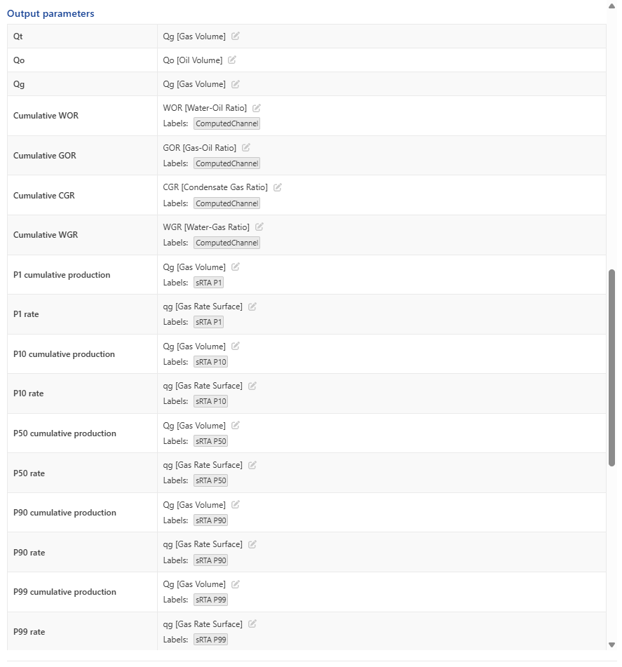
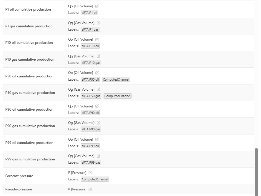
Output datasets
The output is given in the form of properties and custom plots.
Properties: In addition, the diagnostic step generates output which can be viewed if the following properties are defined in the table below. As with the input properties, they are identified by the alias in the user task code. The name is what is visible in the property table and is only for display purposes, hence configurable. Although none of these properties above are mandatory, it is recommended to create them as they may be useful in monitoring the results of the diagnostic and probabilistic forecasts.
Alias | Name | Description | Measure |
|---|---|---|---|
RTA_mQ | mQ | The mQ value of the 1st (inner) zone, as determined by the RTA diagnostic. | No unit |
RTA_mQ_2 | mQ | The mQ value of the 2nd zone, as determined by the RTA diagnostic (if present). | No unit |
RTA_Fractional_Half_Dimension | Fractional half-dimension | The fractional half dimension of the 1st (inner) zone, determined by the diagnostic | No unit |
RTA_Fractional_Half_Dimension_2 | Fractional half-dimension | The fractional half dimension of the 2nd zone, determined by the diagnostic (if present) | No unit |
RTA_Xmf | Xmf | The Xmf as determined from mQ and the | No unit |
RTA_t_star | t* | The t* value as described in URTeC 5096 | Time (hours) |
RTA_Q_star | Q* | The Q* value as described in URTeC 5096 | No unit |
Dimensionless_Wellbore_Storage | Dimensionless wellbore storage | The value of CD deduced from the value of c and Q* | No unit |
RTA_Skin | Skin | The value of skin deduced from the value of b, t* and Q* | No unit |
RTA_XX_Gas_Cum_Production (where “XX” is any of [P1, P10, P50, P90, P99]) | XX gas production | The forecasted cumulative gas production of the well associated with probability XX | Large gas volume |
RTA_XX_Oil_Cum_Production (where “XX” is any of [P1, P10, P50, P90, P99]) | XX oil production | The forecasted cumulative gas production of the well associated with probability XX | Large liquid volume |
Although none of these properties above are mandatory, it is recommended to create them as they may be useful in monitoring the results of the diagnostic.
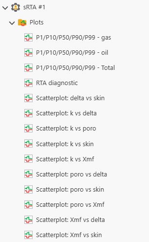
Plots: The sRTA user task creates several custom plots shown in the figure. Note that the probabilistic forecast plots will update automatically when the datasets are updated. The plots are shown in a subfolder, as shown in the figure.
An example of the diagnostic plot is shown below. The straight lines show the fit to the data. The fractional half-dimension is determined from horizontal line through the t/Q dQ/dt values. The mQ value is the slope of the line fitting the Qn values. The diagnostic plot is essential in determining the quality of the initial guesses of the fractional half-dimension and mQ which are given to the sampling procedure.
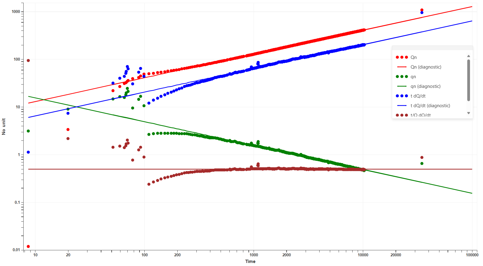
Diagnostic plot
Examples of the probabilistic forecast for total cumulative production is shown in the figure below. These plots show the forecasts conditioned to the total cumulative production. The data (total cumulative production) is determined by the PVT and the cumulative production of each phase. The values are in BOE (for dead oil and black/volatile oil production), or Mcf (for condensate gas or dry gas). The probabilistic forecasts for the cumulative production (oil or gas) are calculated from the cumulative production ratios and the PVT properties.
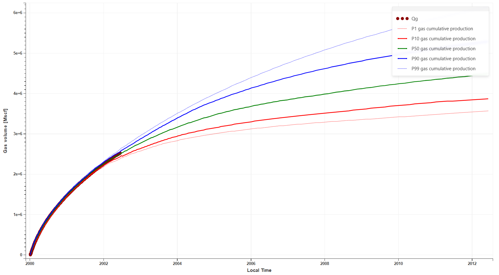
Probabilistic forecast for total cumulative production
An example of the scattergram plot showing the variation of the uncertain parameters is shown below. The scatterplots will show the values of the unknown parameters which were selected by sampling procedure, and any dependence between them.
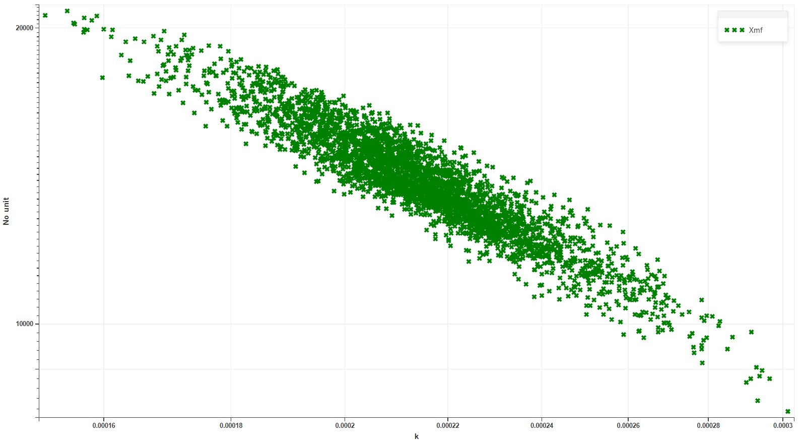
Scattergram plot