Creating aRTM Workflow
The aRTM workflow starts with a PVT object. It can then proceed automatically from a pressure and possible rate feeds. See Automatic RTM for more details.
A PVT object must be extracted under the field or well group.
Definition section
In the field/well group node click on Automatic RTM,
 , under the Info tab:
This will launch the following aRTM dialog:
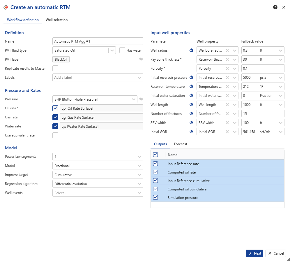
Assign a Name to the aRTM workflow.
Select the PVT fluid type to be used. A PVT label may be specified; otherwise, the first uploaded PVT document is used by default.
Note
The Numerical NL option is automatically activated in the generated files.
This does not affect results; it only facilitates a smoother transition to Numerical NL mode.
Enable Replicate results to copy the results to the master container (This option is not recommended before validating the results, as the master container serves as the repository for validated results.).
Optional. Add a label(s) if necessary.
Note
This label(s) will tag the aRTM outputs and the generated document.
Pressure and Rates sections
Select the type of pressure gauge (P or BHP) to be used and add a label(s) if necessary to make the required binding. Labels input is not offered by default but can be accessed by clicking on
 next to the pressure data type drop down list.
Check the data type that is used for Production channels for this aRTM; the reference phase in will depend on the reference phase in the seed PVT document.
Enable Use equivalent rate when multiple rate phases are present and total extraction is required.
Note
If multiple gauges are selected and this option is disabled, all gauges are copied to the generated file and only the reference phase in the PVT is used for extraction.
Model section
Set the Power law segments.
The Power Law tool estimates the transient flow regime from production data and provides initial estimates for the analytical model parameters.
1 Segment: With 1 Power Law segment, the production behavior is represented by a single power-law relationship over the selected history period. This assumes that the well follows one dominant flow regime throughout the analyzed period.
2 Segments: With 2 Power Law segments, the production history is divided into two periods, each represented by its own power-law relationship.
Select the Analytical model. See Analytical models for more details
Select Improve target
When Rate is selected, the regression algorithm minimizes the difference between the simulated production rate and the measured production rate.
When Cumulative is selected, the regression algorithm minimizes the difference between simulated and measured cumulative production.
When both of them are selected, Objective function is split 50/50 between them.
Select Regression algorithm
Select one or more well events to generate a multiple analysis based on well events. This action enables automatic switching to the corresponding Proxy models and activates the option to create one document per Xmf step. See for Automatic aRTM for more details.
Input well properties section
In the Input well properties section, well properties may be taken from the master container, fallback values, or erased so that PVT parameters are taken directly from the PVT object.
Note
When a well property is selected, the workflow searches for it in the Well Properties master container. The desired properties can be selected.
When a well property column is left empty, the fallback value is used.
When the optional inputs eraser ,
 , is clicked:
Reservoir temperature and Initial GOR are taken from the PVT object.
The reference pressure used in the PVT update is taken from Pi of extraction, not from well properties.
Default values (in Topaze) are used for all other properties.
Well properties values may be provided through:
Well Flat View
Multiwell load
SDK
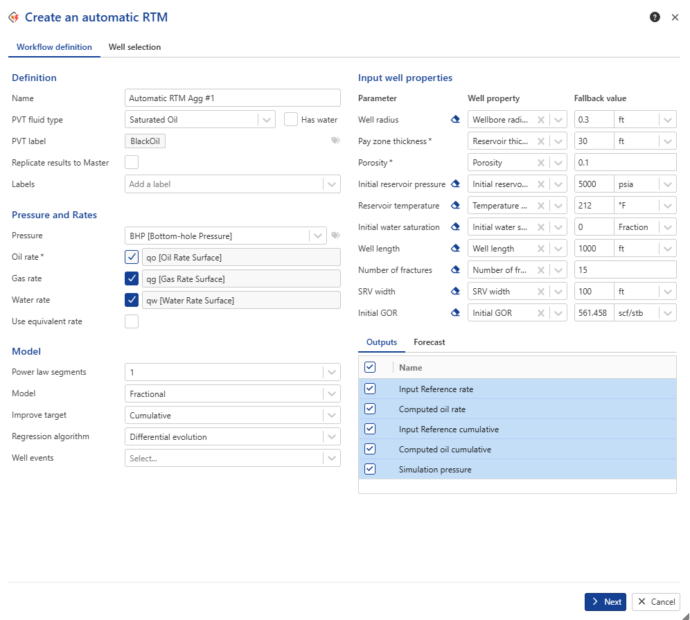
Select the gauges to output.
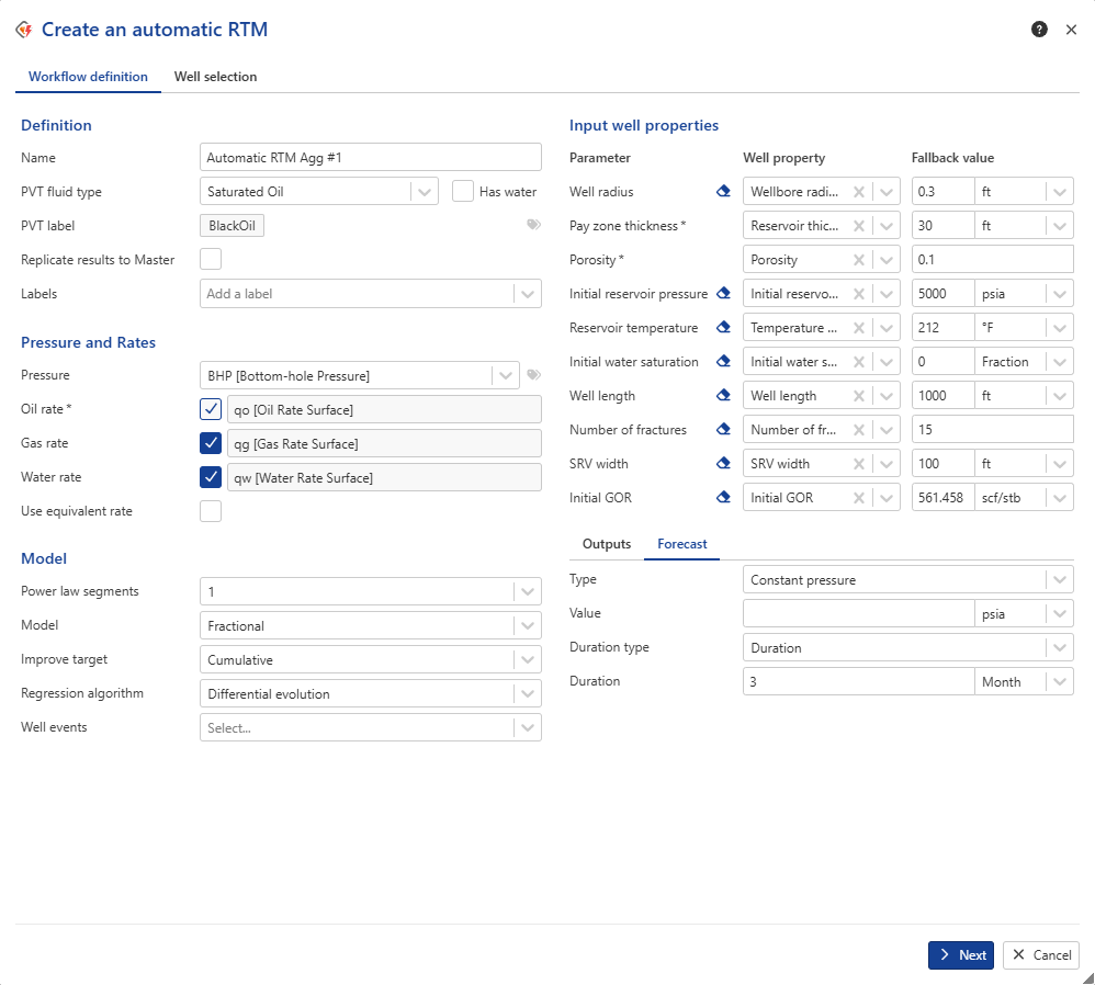
In the Forecast tab, define forecast parameters: Type, Duration and Value.
Note
Three forecast types are available:
Constant pressure: where:
A constant pressure value must be defined.
Three duration options are available:
Duration: forecast duration for each new generated file.
End date: forecast ends at a specified date.
EUR: forecast ends when the abandonment rate is reached (an additional input appears for the abandonment rate)
Constant rate: where:
A constant rate value must be defined.
Three duration options are available:
Duration: forecast duration for each new genertaed file.
End date: forecast ends at a specified date.
Pressure trend: where:
Pressure follows a decline trend.
A slope is automatically computed using a line fit over the last 3 months, requiring at least 10 points.
When this type is selected, the following must be defined:
Minimum and maximum pressure values.
Duration option: End date or Duration (Elapsed time)
Click on next or switch to well seclection tab to select Wells to which you want to apply the aRTM workflow.
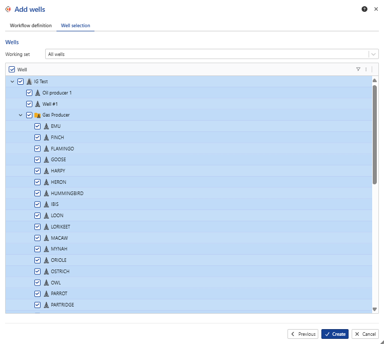
Click on Create .
Model behavior
MZFD
Lw, N, and SRV width are automatically updated if present in the master container.
Permeability is included in regression if at least one of Lw, N, or SRV is present.
Lw is not included in regression.
SRVB and Trilinear
Lw and N are automatically updated if present in the master container.
N is excluded from regression if updated from well properties.
Lw is not included in regression.
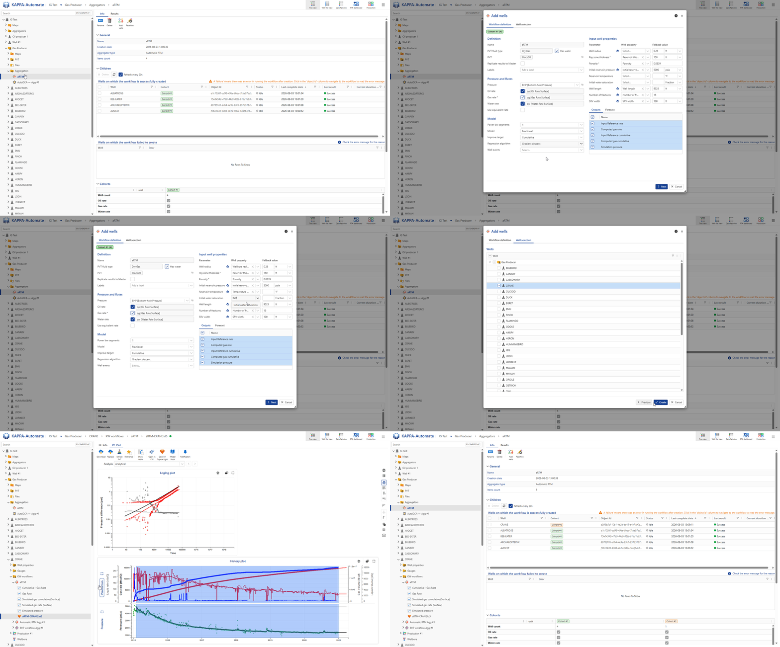
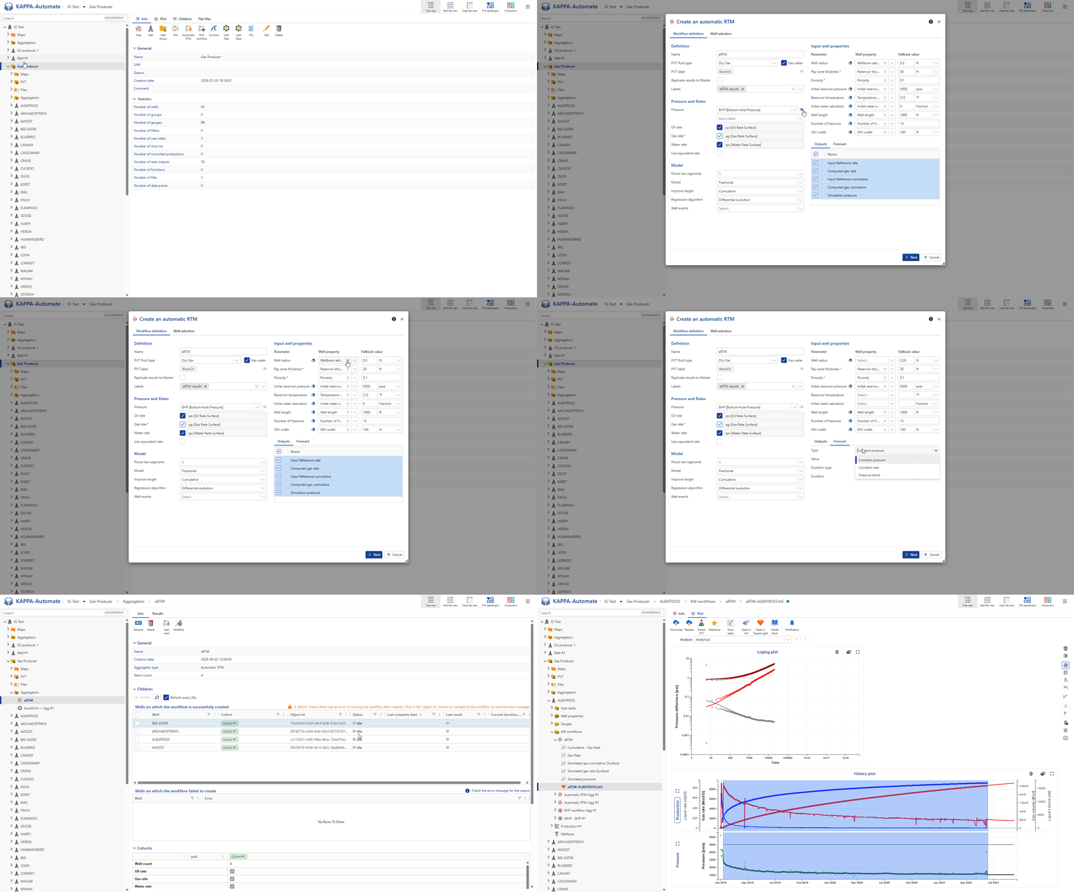
All steps are shown in the .gif below.
Add a new well to an aggregator
A well can be added to an existing aggregator, with the limitation that only wells may be added; other existing inputs in the aggregator cannot be modified. To proceed:
Under the relevant field or well group, select the Aggregator to be updated.
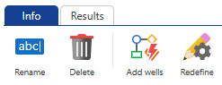
in Info page, click on Add wells option ,
.
Select the cohort group input to initialize from; the input can be edited if required.
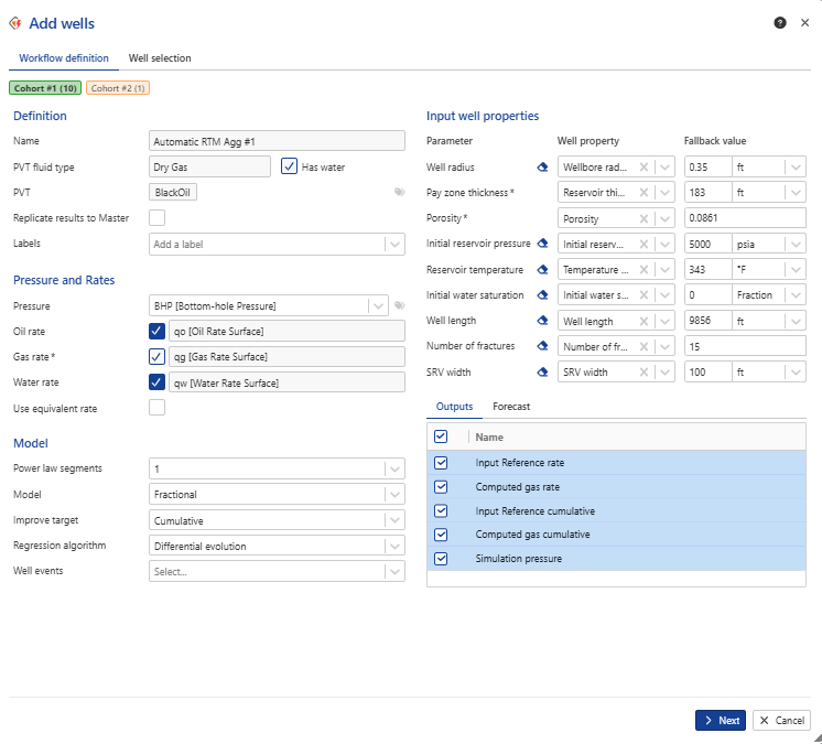
Select the well(s) to include.
Click on Create.
All steps are shown in the .gif below.