Pressure Drop Models and Correlations

The Drift-flux models represent multiphase flow in wellbores or pipes in terms of a number of empirically determined parameters. The great advantage of this model is that there is a continuity between the various flow regimes.

The basic output of the model is the velocity/hold up of each phase. Once known, the hold ups can be used to determine the average segment fluid properties which can then determine the frictional, hydrostatic and acceleration components of the pressure drop.

Three variants of the model are offered: Liquid-gas, Liquid-liquid, 3-Phases.

The model divides a 3-phase system in to a liquid-gas system first to determine gas and liquid hold ups. Once the liquid hold up is determined, the oil-water system is resolved to determine oil and water hold ups.

2-Phase Liquid-Gas

The gas velocity is related to the mixture velocity by the equation:

Where C and vd are the profile parameter and the drift velocity respectively. Correlations exist for the determination of each.

2-Phase Liquid-Liquid

The oil velocity is related to the mixture velocity by the equation:

Where C' and v'd are the profile parameter and the drift velocity respectively. Correlations exist for the determination of each.

3-Phase Model

To model three-phase flow, a two-stage approach is first applied based purely on the two-phase flow models. The system is first treated  as a gas-liquid flow to determine the gas hold up and then model the liquid as an oil-water system to determine the liquid hold ups. To account for the affect of gas on the oil-water slippage for deviated wells however, the model uses different coefficients for the empirical correlations compared to the 2-phase models.

In 1965, Hagedorn and Brown published a correlation for calculating pressure gradients in wells flowing multiphase fluids. The correlation was developed from 475 tests obtained from a 1,500-ft test well at Dallas, Texas, along with 106 tests reported by Fancher and Brown. The combined data resulted in 2,905 pressure measurements. The test well used by Hagedorn and Brown was completed with two separate casing annuli to allow the injection of gas through a gas lift valve near 1,400-ft and liquid through the bottom of the tubing string. Pressure readings were obtained at four points along the tubing string using surface readout gauges mounted on the tubing. Temperature throughout the well was constant at 80°F. The ranges of the data are:

No flow-map was developed. The heart of the method is the single liquid holdup correlation provided for all conditions.

Since the original Hagedorn and Brown correlation was published, several modifications have been proposed. Among these include a restriction limiting the liquid holdup to values greater than the no-slip holdup, and the inclusion of the Griffith and Wallis correlation for the bubble flow regime. This can be activated by checking the Bubble flow add-on option for the correlation.   The Hagedorn-Brown method is seen to over predict the pressure loss for heavier oils (13-25 °API) and under predict the pressure profile for lighter oils (40-56 °API). The pressure drop is over predicted for GLR greater than 5000. Pressure drop has also been observed to be over predicted for tubing sizes greater than 1.5 in.

Reference: "Experimental Study of Pressure Gradients Occurring During Continuous Two-Phase Flow in Small Diameter Vertical Conduits", Hagedorn, A.R., & Brown, K.E., JPT (April 1965), Vol. 17, p. 475.

"Two-Phase Slug Flow", Griffith, P. and Wallis, G.B., J. Heat Transfer; Trans. ASME (Aug. 1961) 307-320.

As an attempt to provide an explicit relation to estimate z-factor, Beggs and Brill presented a closed form expression. The method adopted an empirical/explicit approach and the correlation is commonly recognized to be of a relatively lower accuracy, except at moderate pressures and temperatures.

Beggs and Brill reported using 94 data points in the development of the correlation which can only be used in the following range

Beggs and Brill reported and average absolute error of 0.19%.

Reference: “Two-Phase Flow in Pipes”, Brill, J. P. and Beggs, H. D., U of Tulsa, INTERCOMP Course, The Hague, Tulsa, OK (1974)

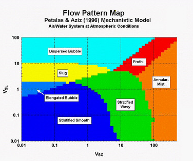
The Petalas and Aziz mechanistic model was not built for a specific set of data or fluid properties. Instead, the authors applied first principles to the possible flow patterns that can be observed at different inclinations. For this reason, it is applicable to any pipe inclination and fluid properties. The model was developed using subsets of a database of over 20,000 laboratory measurements and data from approximately 1,800 wells.

The model distinguishes the following regimes:

Stratified flow regimes are restricted to horizontal flow.

The method could be summarized as follows:

With the continuous evaluation of the stability of the flow patterns, the corresponding flow pattern map to the given flowing conditions can be created. The following is a typical flow pattern map for vertical upward gas-oil flow:

Reference: "Development and Testing of a New Mechanistic Model for Multiphase Flow in Pipes ", Petalas N., and Aziz, K., ASME Fluids Engineering Division Second International Symposium on Numerical Methods for Multiphase Flows, San Diego, Cal., July 7-11, 1996.

In 1984, Reinicke, et al published a method for calculating pressure gradients in high-water cut gas wells. They initiated a study to determine a method for calculating the pressure drop for wells completed in the Rotliegendes gas formation in Germany. The study arrived at the following conclusions concerning multiphase flow correlations:

A total of 70 tests from 26 wells encompassing the following ranges were used in the study.

The data was grouped into mist flow, possible mist flow and non-mist flow. A hybrid correlation involving the Duns and Ros mist flow model and Gray's correlation resulted. The following graph shows the flow pattern map used to define the slug-transition-mist flow regimes:

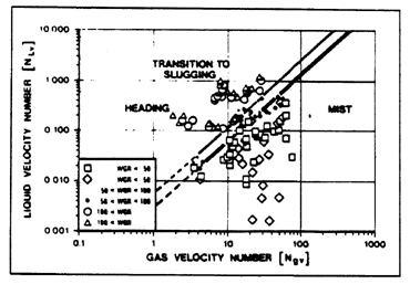Since this correlation was developed using field data acquired from wells in mist or near-mist flow conditions, it is not expected to work well for wells in the bubble-slug flow regimes.

Reference: "Comparison of Measured and Predicted Pressure Drops in Tubing for High-Water-Cut Gas Wells", Reinicke, K. M., Remer, R. J. and Hueni, G., SPE 13279.

Gray's correlation was published in 1978 as part of the API computer program for sizing subsurface safety valves. The method was developed from 108 selected gas well tests of which 88 reportedly produced free liquids. Since the correlation was primarily developed for vertical gas-condensate wells, it usually predicts smaller values of liquid holdup than the other pressure gradient correlations. As a result of limits in the well data used for developing the correlation, Gray pointed out that it should be used with caution for the following conditions:

Despite these restrictions however, the correlation has been successfully used with oil wells.

Reference: "Vertical Flow Correlation - Gas Wells", Gray, H. E., User Manual for API 14B, SSCSV Sizing Computer Program, App. B (Jan 1978) 38-41.