Automatic DCA (aDCA)

Overview

This user task is designed to calculate an Arps or Modified Hyperbolic decline curve fit to oil and gas production for a well. The task can take as input one or more well properties as well events which determine when a decline curve starts. A new forecast will be performed when a new well event occurs, as well as when a user-specified amount of new production data is added to the well. Optionally, the task can automatically calculate change points where a new decline curve will start. If there are no well events and the automatic change point calculation is not selected, the user task will use the date corresponding to the maximum rate as the initial point for DCA.

The user task always performs an optimization procedure to obtain a best fit to the selected decline curve. A forecast is always perform to a specified abandonment rate, or up to a maximum lifetime of the well. Optionally, the user task can also perform the Nested Sampling procedure, which performs tens of thousands of function evaluations to calculate a Bayesian probabilistic forecast.

When a secondary phase (oil or gas) is specified as input, that phase is modeled as a function of the primary phase via the following power-law relationship:

G_p = G_p^intN_p^m

where G_p is the cumulative production of the secondary phase, N_p^m is the cumulative production of the primary phase, G_p^intis the intercept and m is the slope of the line fit on the log-log plot. Before dropping below bubble point or dew point, m=1 and G_p^intint equals the initial GOR/CGR. Since at the bubble point the cumulative production of the secondary phase is the same, there are three unknown variables to fit to the data: the initial GOR/CGR, the slope post-bubble/dew point, and the time at which the well reaching bubble/dew point. These are the three parameters which are employed in the optimization and sampling procedures to obtain a match of the secondary phase production.

The outputs from the user task are displayed in the “Plots” folder found under the user task node for the well. In addition to the plots and associated datasets, the user task outputs several well properties if K-A is configured to store them (see Prerequisites, below). Specifically, the task stores for each forecast the best fit and (if probabilistic forecast is selected) Bayesian posterior parameters for the Arps or MH equations and the EUR for oil and/or gas production. In addition to the usual rate and cumulative production output, the user task calculates and outputs the nominal decline (D) and the b-factor for the data and model outputs. The derivatives are calculated using log-cycle spacing in time (value of 0.1).

The user task offers the option to match on pressure-normalized rate (PNR), also known as PNR-DCA. In this case, the user task requires an input of pressure. If it is a gas well, a PVT object is also required. The initial pressure is obtained from the well property with alias MainResult_InitialPressure, or, if not initialized, the maximum value in the pressure dataset. For the moment, the PNR-DCA option does not allow for a secondary phase. In this option, the Arps or MH parameters are fitted to the PNR, not the rate. The q vs time plots will not be created – only the rate/PNR vs cumulative production.

Theory

Arps Arps hyperbolic decline:

In its simplest form, the rate specified at a given time is expressed as:

Equation 14.

q=\frac{qi}{\left(1+bat\right)^{\frac{1}{b}}}

Where:

qi: the Initial Rate

b: the b exponent

Di: the Nominal or Instantaneous Decline Rate

When b = 0, an exponential decline is observed and the general hyperbolic equation simplifies to:

Equation 15.

q=qie^{-Dit}

When b = 1, a harmonic decline is observed and the general hyperbolic equation simplifies to:

Equation 16.

q=\frac{qi}{\left(1+Dit\right)}

Modified hyperbolic equation:

Transition Time: The transition from hyperbolic to exponential occurs when instantaneous decline rate equals the terminal decline rate:

Equation 17.

D\left(t^{\cdot}\right)=\frac{Di}{1+bDit^{\cdot}}=D\lim

Solving for t*:

Equation 18.

t\cdot=\frac{1}{bDi}\left(\frac{Di}{D\lim}-1\right)

This can be simplifeid to:

Equation 19.

t\cdot=\frac{Di-D\lim}{bDiD\lim}

Prerequisites

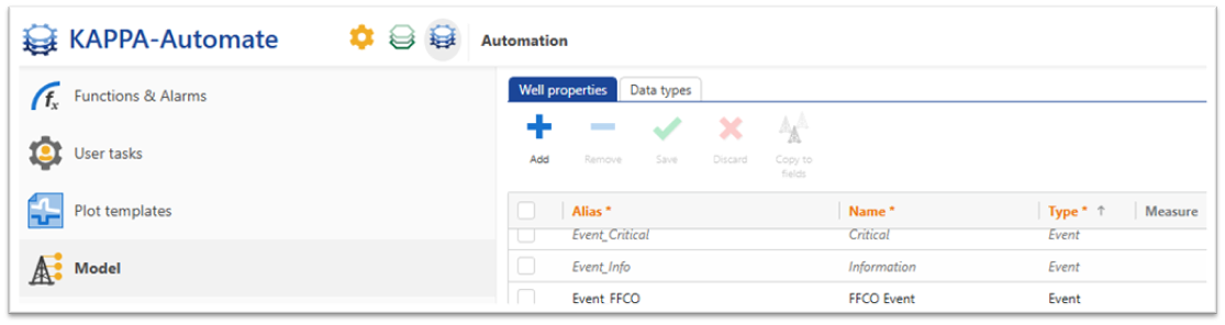
Well events: The AutoDCA user task can take as input one or more well properties which indicate dates of workovers, choke changes, and other events where a new decline curve should be fitted to the wells. Before creating the AutoDCA user task, the well events must first be specified in the global list of well properties. The global list of well properties can be seen under the “Automation” view, in the “Well properties” tab (shown in the figure below). These well events can be specific to the company and must of type “Event”. Well properties are identified by a unique alias, shown in the first column of the well property table below

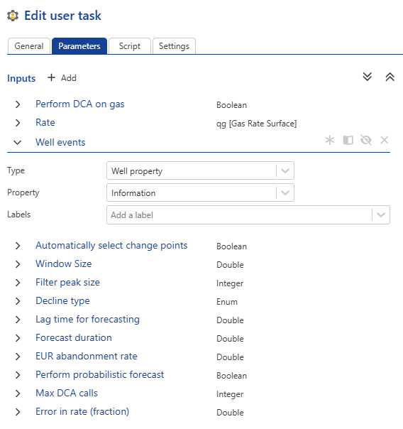
When defining the AutoDCA task in K-A, you must set up the well event input in the Parameters tab as shown in the figure below. In the figure below, there is a single input of Type “Well property” which defines the well events, entitled “Well events” (highlighted). Note however that more than one input for well events is allowed. The Property dropdown box in the UI (highlighted) corresponds to the “Name” of the well event (the second column in the table above). Note that the property name is what is visible in the property table and is used only for display purposes, hence configurable.

Well properties The Auto DCA user task also outputs well properties which are optional but recommended to take full advantage of the user task. These well properties are described in the table below.

Well property	Alias	Measure	Description
Average Arps Di decline	DCA_Average_Arps_Di_Decline	Inverse time	Arps Di decline rate value from best fit, or weighted arithmetic average of Di from sampling if performing probabilistic forecast
Percentile Arps b decline	DCA_{percentile}_Arps_Di_Decline	Inverse time	Replace the tag {percentile} by P1, P10, P50, P90, and P99. This property represents the percentile of the Arps Di decline rate calculated from sampling if performing a probabilistic forecast.
Percentile Arps b exponent	DCA_{percentile}_Arps_ b_Exponent	No unit	Replace the tag {percentile} by P1, P10, P50, P90, and P99. This property represents the percentile of the Arps b exponent calculated from sampling if performing a probabilistic forecast.
Percentile Cumulative Phase Forecast	DCA_Average_Cumulative_{phase}_Production	Gas or liquid volume	Replace the tag {phase} by either oil or gas. This property represents the cumulative production up to the end time of the forecast, including the historical production. The value is calculated from the best fit curve, or from a weighted arithmetic average from the sampling.
PAverage EUR Cumulative Phase	DCA_ Average_EUR_Cumul_{phase}	Gas or liquid volume	Replace the tag {phase} by either oil or gas. This property represents the cumulative EUR, including the historical production. The EUR is calculated from the best fit curve, or from a weighted arithmetic average from the sampling. The input value to “EUR abandonment rate” is used as the final rate to calculate the EUR. If this value is not specified, then the default value is 0.01 times the maximum historical rate.
Average Cumulative Phase Prod Forecast	DCA_{percentile} _Cumulative_{phase}_Production	Gas or liquid volume	Replace the tag {percentile} by P1, P10, P50, P90, and P99. This property represents the percentile value of the cumulative production up to the end time of the forecast, including the historical production, as determined from the sampling procedure. Consequently, the values are calculated only when a probabilistic forecast is performed.
Percentile EUR Cumulative Phase	DCA_ {percentile}_EUR_Cumul_{phase}	Gas or liquid volume	Replace the tag {percentile} by P1, P10, P50, P90, and P99. This property represents the probabilistic cumulative EUR, including the historical production. The input value to “EUR abandonment rate” is used as the final rate to calculate the EUR. If this value is not specified, then the default value is 0.01 times the maximum historical rate. The values are calculated only when a probabilistic forecast is performed.
Average Arps b exponent	DCA_Average_Arps_b_Exponent	No unit	Arps b exponent from best fit, or weighted arithmetic average of b from sampling if performing probabilistic forecast

Input

This section describes the input to run the AutoDCA user task. The description of each user task input is provided in the table below

Perform DCA on gas - Boolean indicated whether gas or oil is the main phase.
Rate - The dataset which contains the rate data (gas or oil).
(One or more well events) - As described in the “Prerequisites” section above, the user task can be configured to accept one or more well properties of type “Event”, indicating when significant well events occurred to start a new decline curve analysis. This can be empty.
Automatically select change points - Boolean to indicate whether the user task should automatically detect and use change points to determine when to start a decline curve analysis.
Window Size - Only showing if “Automatically select change points” is true. Controls the amount of detail in the analysis of the rate curve. In general, the smaller the window size, the more change points will be detected.
Filter peak size - A non-negative number indicating the number of consecutive points to treat as peaks or valleys. If this value is > 0, the user task will attempt to filter out extreme peaks (valleys) in the rate curve to remove potentially anomalous rate values.
Lag time for forecasting - The amount of time that the user task will wait until performing another DCA calculation.
Forecast duration - Duration of forecast beyond the last data point recorded.
Perform probabilistic forecast - If true, the user task will perform a probabilistic forecast. Otherwise, a one-curve, best fit will be performed.
Max DCA calls - Only visible when “Perform probabilistic forecast” is true. Often unnecessary to modify unless the forecast does not appear to converge correctly, or if the calculations are taking too long.
Error in rate (fraction) - Only visible when “Perform probabilistic forecast” is true. Controls the error tolerance around the rate data.

Output

The user task outputs several datasets, described in the table below.

Decline points - This dataset indicates the location of the change points, which are either derived from the well event input(s), and/or the automatic selection.
Filtered rates - The filtered rates which occur when “Filter peak size” is positive.
P1/P10/P50/P90/P99 - The output of the decline curve fit. When performing deterministic forecasts, only the P50 output will be employed and will represent the best fit. When performing a probabilistic forecast, all percentiles will contain output and are a reflection of the curves and the input error fraction.

Automatic DCA user task definition

Procedure

At the well level, click on User Task ,, from the top options.
In the user tasks list, select Auto DCA.
Assign another name to the user task, if required.
Check perform DCA on gas if gas phase DCA is required.
Check perform PNR-DCA, if checked a BHP channel is required.
Select the decline type.
Select the main phase and the second phase (optional).
Select one or more well events.
Check select change point; if enabled, the user task detects and uses change points to determine when to start the decline‑curve analysis.
Adjust the filter peak size, if needed.
Set the lag time for forecasting, if needed; this represents the amount of time the user task waits before performing another DCA calculation.
Set the maximum well life (this includes well data + forecast duration; if the duration is shorter than the data length, no forecast will be generated).
Input EUR value.
Check perform probabilistic forecast to generate multiple forecasts; if enabled, three additional inputs appear and can be adjusted in case of convergence issues:
- Max DCA calls
- Error in rate (fraction)
- Error in secondary rate (fraction)
Define the output data types and labels, if required.
Click Create.

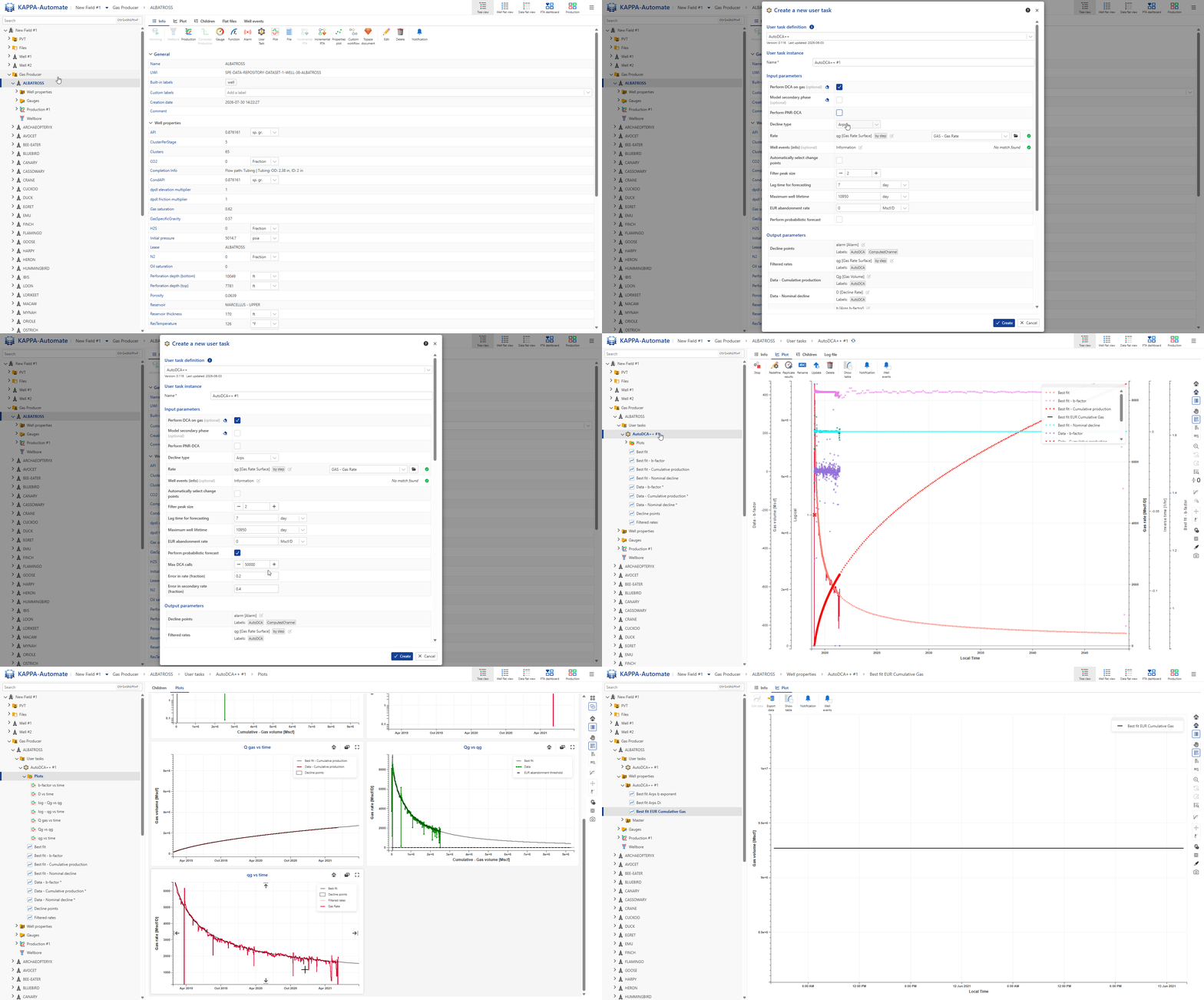
All steps are shown in the .gif below.

In this section:

K-A End User Help

Automatic DCA (aDCA)

Automatic DCA user task definition

Search results