Production Dashboard
The Production Dashboard provides an integrated workspace for visualizing and managing production data across multiple wells within a field. It enables users to plot production trends from various wells on multiple graphs within a single interface, allowing for easy comparison and quick analysis.
In addition to visualization, the dashboard supports bulk operations such as applying functions, running user tasks, and executing workflows like aRTM and BHP conversions. Model results can also be displayed directly from the same workspace.
An interactive map and a well properties table can be included, providing a complete and centralized overview of the field’s performance.
Production and pressure must exit under the well (s).
Select the Field in the hierarchy.
Click on the Production Dashboard,
 , option in the top right toolstrip.
Select a working set from the dropdown list.

Important
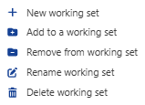
To manage new working set, click on
 :
:To create a new working set click on
 .
.To add wells to a working set click on
 .
.To remove wells from working set click on
 .
.To rename an existing working set click on
 .
.To delete a working set click on
 .
.
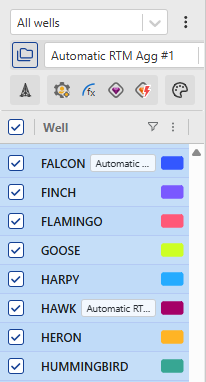
Select the well(s) to be included in the dashboard.
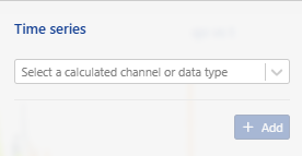
Click on
 to open the time series dialog and select data types to display. Two channel types are available:
Calculated channels: computed on the fly (e.g., Productivity Index)
Data channels: directly plotted from existing data. (e.g., pressure, rates).
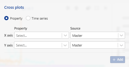
Click on
 to open the cross plot dialog.
Select:
Data type (properties or time series)
X‑axis variable
Y‑axis variable
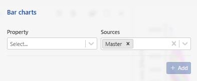
Click on
 to open the well properties bar chart dialog.
Select well properties to display (e.g., gas specific gravity, dew‑point pressure).
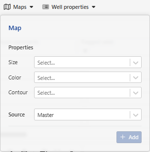
Add maps by clicking on
 .
.One or multiple maps can be created with custom configurations (size, color, contour). These configurations use the Well Properties Container without affecting maps defined in the tree view.
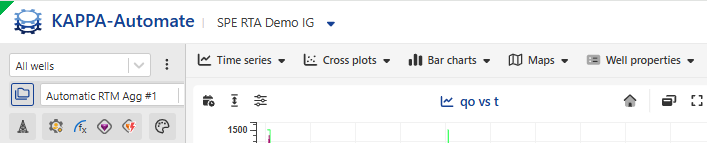
From the toolstrip, various data types can be displayed as plots, along with well properties sourced from a defined container.
Select the Main Phase:
If Gas is selected, the calculated PI is gas PI.
If Oil is selected, both oil PI and liquid PI are calculated.
Productivity Index (PI) Calculation
PI is calculated on the fly using:
Equation 1.where:
Qi: the rate at step i
Pi: the iniltial pressure
P(i): Pressure at step i.
GOR and WC ratios can be plotted versus:
Liquid cumulative volume (if main phase is oil)
Gas cumulative volume (if main phase is gas)
Enable the Results option to add a results table.
A result container can be selected for each well.
Activating the Master container results option displays a unified table of well properties sourced from the master container.
Tip
Plot scaling and display options are available in the right-hand side vertical toolbar. See Plot Scaling and Display Options
Bulk operations
At the top of the wells table, you can perform bulk operations on the selected wells:
Select aggregator container results using
 .
.Run a user task by clicking

Apply functions in bulk using

Execute the BHP workflow in bulk via

Run the aRTM workflow in bulk using

Switch to single well selection using

Result view
The dashboard displays a combined view of all selected wells and plots. Several display configurations are possible:
Examples:
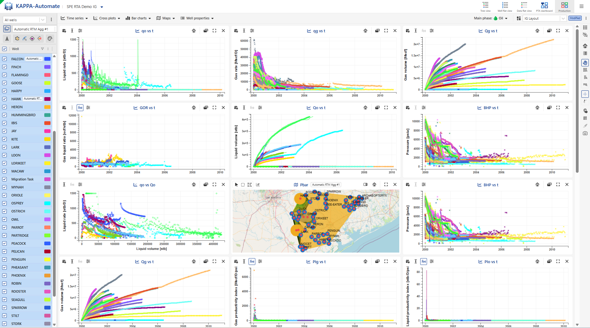
1- Plots with Data Types
This configuration shows production plots alongside time series channels, calculated channels, and any some data types selected from the catalog.
 |
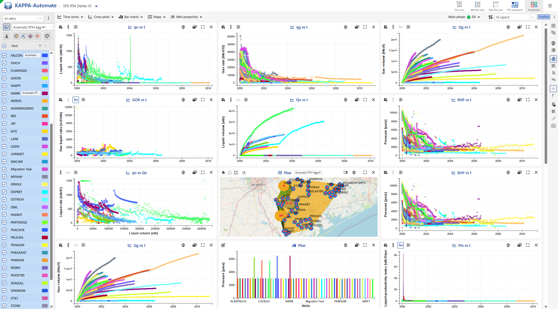
2- Plots with Templates and Bar Charts
When templates and well‑property bar charts are added, the dashboard displays both dynamic plots and static property comparisons.
 |
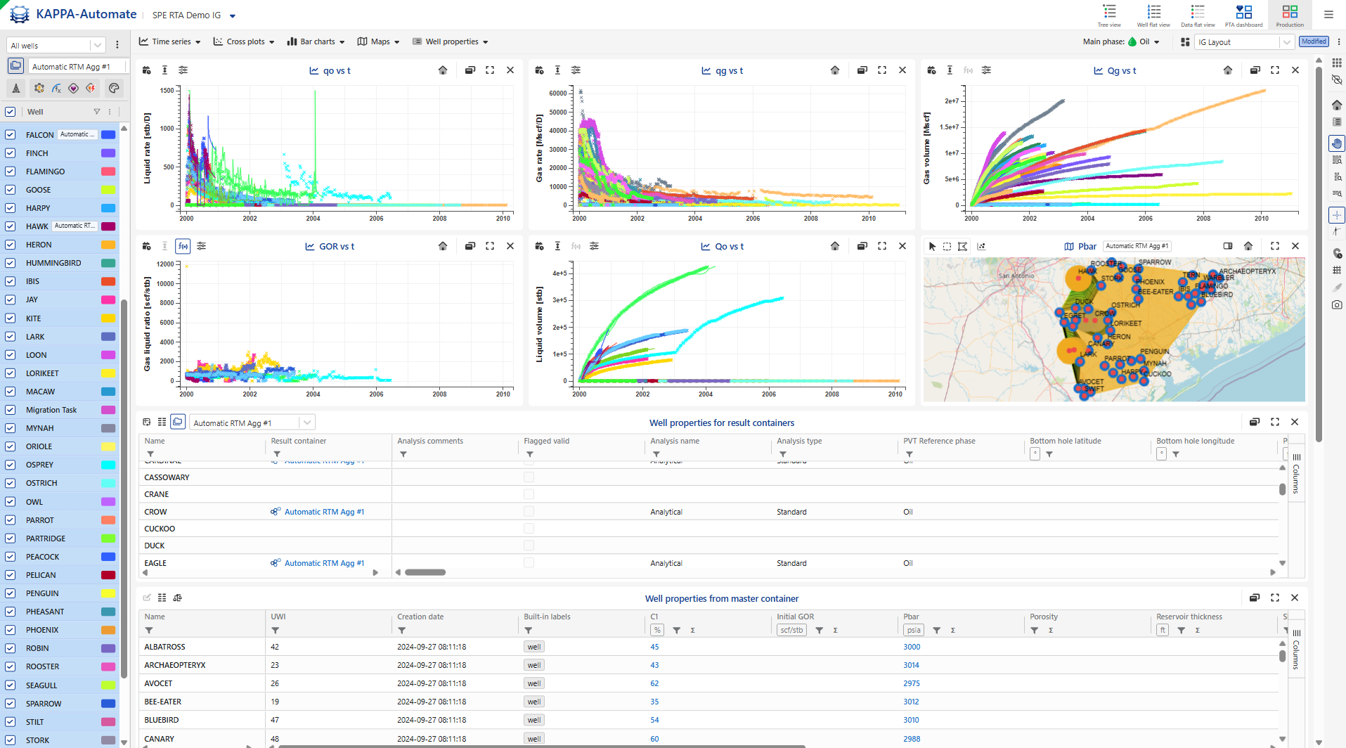
3- Plots with Well Properties Tables
A well properties tables can be added to complement the plots, providing a structured overview of key parameters for each well.
 |
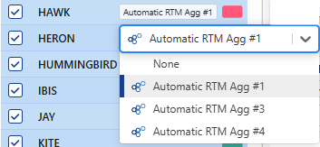
Wells color can be modified directly from the well table. Click the colored box next to the well name to select a new color.
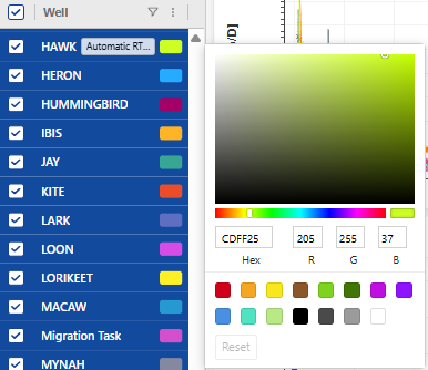
The results container can also be changed by clicking the label that displays the workflow name. This opens the list of all available results.
 |
Defining Layout
The Production Dashboard supports saving and managing custom layouts, allowing consistent visualization across sessions or sharing configurations with other users.
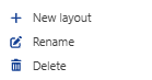
Open the layout menu by clicking on
.Select New layout.
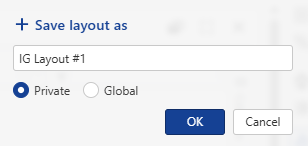
Provide a layout name and choose the storage mode:
Private: saved locally on the machine.
Global: saved in the database and shared with all users.
Once saved, layouts can be renamed using
or deleted using .When the dashboard configuration is changed (e.g., plot order modified, plots added or removed), a Modified
 notification appears:
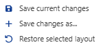
Clicking the notification opens a dialog offering three actions:
Save changes: update the existing layout.
Save as new layout: create a new layout while preserving the original.
Restore layout: discard modifications and revert to the saved layout.
To load an existing layout:
Click on

Select the desired layout from the list.
Layouts can also be restricted to the current field, ensuring that the selected layout is automatically applied whenever the field is accessed.
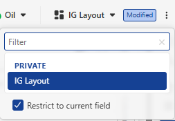
Table options
Pivot option
 , swap between columns and rows
Show only values with values using
 .
.Show results container in the plot using
and select the container from the dropdown list.Apply a single unit for all properties sharing the same measure

Plot options
On individual plots, time scales can be switched using the (accessible through the Absolute,
 , option), The available scales include:
Absolute time: represents the original date.
Production time: represents the time elapsed from the first rate.
Time from peak rate: represents the time elapsed from the maximum rate. The reference phase rate should then be selected.
Time on production: represents the time elapsed from the first rate, with shut-in periods excluded.
Note
Time scales such as production time, time from peak rate, and time on production are defined based on the selected phase.
Production rates can be normalized on individual plots using the normalize
 option). Available normalization methods include:
Oil cumulative production at 6 months (with or without using a reference well).
Gas cumulative production at 6 months (with or without using a reference well).
Well property (with or without using a reference well).
If measured data are missing, channels can be computed directly on individual plots using the

On individual plots, the scale can be switched between linear and logarithmic by clicking the ,
 , and selecting the desired axis (X or Y).
Reset zoom using the reset option
 .
.Remove a plot using the Remove option ,
 .
.Open a plot in a separate window using ,
 .
.Expand or restore plots using the Maximize ,
 , and Minimize ,
 , options.
Toggle between Default and Compact layouts by clicking on
 .
.The X-axis can be synchronized by clicking on
.Zoom an individual plot using Ctrl + mouse wheel.
Map options can be accessed by clicking on
 option.
Wells can also be selected directly from the map options:
Sigle click selection ,
 .
.Rectangular selection ,
 .
.Polygon selection ,
 .
.
Add/remove table columns by clicking on
 at the right of the table.
Highlight individual wells on all plots by clicking on them in the well list, the plots, or the map.
Highlight multiple wells on all plots:
CTRL or Shift key: select wells from the table and plots
Shift key: select wells from the map
All the features described above are illustrated in the .GIF below.